

16 Strain Gradient Models for Growing Solid Bodies
283
D
Dt
t
ρdx =
t
Dρ
Dt
+ ρ∇.v
dx =
t
π dx +
∂∂ t
mds ≡
t
ρdx
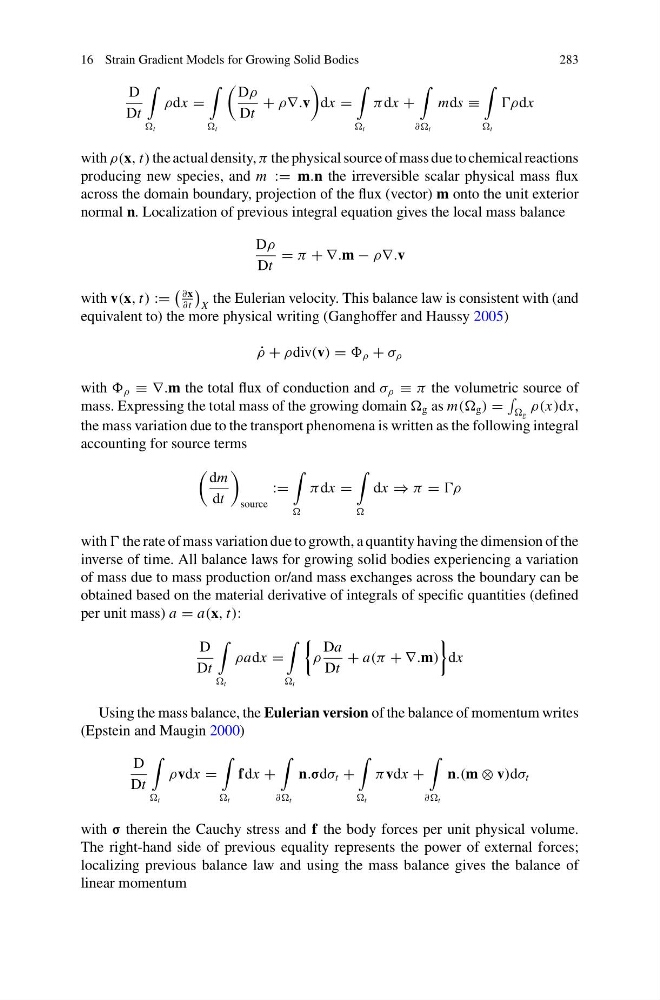
with ρ(x, t) the actual density, π the physical source of mass due to chemical reactions
producing new species, and m := m.n the irreversible scalar physical mass flux
across the domain boundary, projection of the flux (vector) m onto the unit exterior
normal n. Localization of previous integral equation gives the local mass balance
Dρ
Dt
= π + ∇.m − ρ∇.v
with v(x, t) :=
∂x
∂t
X
the Eulerian velocity. This balance law is consistent with (and
equivalent to) the more physical writing (Ganghoffer and Haussy 2005)
˙
ρ + ρdiv(v) = ρ + σ ρ
with ρ ≡ ∇.m the total flux of conduction and σ ρ ≡ π the volumetric source of
mass. Expressing the total mass of the growing domain g as m(( g ) =
g
ρ(x)dx,
the mass variation due to the transport phenomena is written as the following integral
accounting for source terms
dm
dt
source
:=
π dx =
dx ⇒ π = ρ
with the rate of mass variation due to growth, a quantity having the dimension of the
inverse of time. All balance laws for growing solid bodies experiencing a variation
of mass due to mass production or/and mass exchanges across the boundary can be
obtained based on the material derivative of integrals of specific quantities (defined
per unit mass) a = a(x, t):
D
Dt
t
ρadx =
t
ρ
Da
Dt
+ a(π + ∇.m)
dx
Using the mass balance, the Eulerian version of the balance of momentum writes
(Epstein and Maugin 2000)
D
Dt
t
ρvdx =
t
fdx +
∂∂ t
n.σdσ t +
t
π vdx +
∂∂ t
n.(m ⊗ v)dσ t
with σ therein the Cauchy stress and f the body forces per unit physical volume.
The right-hand side of previous equality represents the power of external forces;
localizing previous balance law and using the mass balance gives the balance of
linear momentum
283
D
Dt
t
ρdx =
t
Dρ
Dt
+ ρ∇.v
dx =
t
π dx +
∂∂ t
mds ≡
t
ρdx
with ρ(x, t) the actual density, π the physical source of mass due to chemical reactions
producing new species, and m := m.n the irreversible scalar physical mass flux
across the domain boundary, projection of the flux (vector) m onto the unit exterior
normal n. Localization of previous integral equation gives the local mass balance
Dρ
Dt
= π + ∇.m − ρ∇.v
with v(x, t) :=
∂x
∂t
X
the Eulerian velocity. This balance law is consistent with (and
equivalent to) the more physical writing (Ganghoffer and Haussy 2005)
˙
ρ + ρdiv(v) = ρ + σ ρ
with ρ ≡ ∇.m the total flux of conduction and σ ρ ≡ π the volumetric source of
mass. Expressing the total mass of the growing domain g as m(( g ) =
g
ρ(x)dx,
the mass variation due to the transport phenomena is written as the following integral
accounting for source terms
dm
dt
source
:=
π dx =
dx ⇒ π = ρ
with the rate of mass variation due to growth, a quantity having the dimension of the
inverse of time. All balance laws for growing solid bodies experiencing a variation
of mass due to mass production or/and mass exchanges across the boundary can be
obtained based on the material derivative of integrals of specific quantities (defined
per unit mass) a = a(x, t):
D
Dt
t
ρadx =
t
ρ
Da
Dt
+ a(π + ∇.m)
dx
Using the mass balance, the Eulerian version of the balance of momentum writes
(Epstein and Maugin 2000)
D
Dt
t
ρvdx =
t
fdx +
∂∂ t
n.σdσ t +
t
π vdx +
∂∂ t
n.(m ⊗ v)dσ t
with σ therein the Cauchy stress and f the body forces per unit physical volume.
The right-hand side of previous equality represents the power of external forces;
localizing previous balance law and using the mass balance gives the balance of
linear momentum