

13 High Strain Rate Tension Experiments Features …
213
σ z (r ) = σ real ·
1 + ln
a
2
+ 2a R − r
2
2a R
,
σ r (r ) = σ θ (r ) = σ real · ln
a
2
+ 2a R − r
2
2a R
.
Distribution of axial and radial stresses for the radius of the minimal neck section
according to Shepinsky obeys the following laws:
σ z (r ) = σ real · exp
a
2
− r
2
2a R
,
σ r (r ) = σ θ (r ) = σ real ·
exp
a
2
− r
2
2a R
− 1
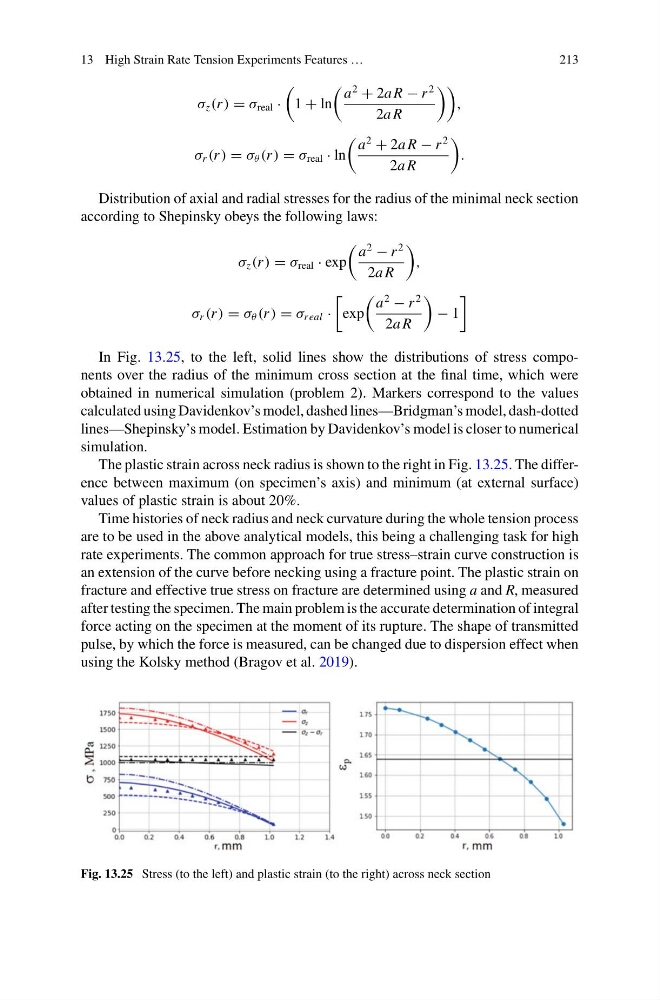
In Fig. 13.25, to the left, solid lines show the distributions of stress components over the radius of the minimum cross section at the final time, which were
obtained in numerical simulation (problem 2). Markers correspond to the values
calculated using Davidenkov’s model, dashed lines—Bridgman’s model, dash-dotted
lines—Shepinsky’s model. Estimation by Davidenkov’s model is closer to numerical
simulation.
The plastic strain across neck radius is shown to the right in Fig. 13.25. The difference between maximum (on specimen’s axis) and minimum (at external surface)
values of plastic strain is about 20%.
Time histories of neck radius and neck curvature during the whole tension process
are to be used in the above analytical models, this being a challenging task for high
rate experiments. The common approach for true stress–strain curve construction is
an extension of the curve before necking using a fracture point. The plastic strain on
fracture and effective true stress on fracture are determined using a and R, measured
after testing the specimen. The main problem is the accurate determination of integral
force acting on the specimen at the moment of its rupture. The shape of transmitted
pulse, by which the force is measured, can be changed due to dispersion effect when
using the Kolsky method (Bragov et al. 2019).
Fig. 13.25 Stress (to the left) and plastic strain (to the right) across neck section
213
σ z (r ) = σ real ·
1 + ln
a
2
+ 2a R − r
2
2a R
,
σ r (r ) = σ θ (r ) = σ real · ln
a
2
+ 2a R − r
2
2a R
.
Distribution of axial and radial stresses for the radius of the minimal neck section
according to Shepinsky obeys the following laws:
σ z (r ) = σ real · exp
a
2
− r
2
2a R
,
σ r (r ) = σ θ (r ) = σ real ·
exp
a
2
− r
2
2a R
− 1
In Fig. 13.25, to the left, solid lines show the distributions of stress components over the radius of the minimum cross section at the final time, which were
obtained in numerical simulation (problem 2). Markers correspond to the values
calculated using Davidenkov’s model, dashed lines—Bridgman’s model, dash-dotted
lines—Shepinsky’s model. Estimation by Davidenkov’s model is closer to numerical
simulation.
The plastic strain across neck radius is shown to the right in Fig. 13.25. The difference between maximum (on specimen’s axis) and minimum (at external surface)
values of plastic strain is about 20%.
Time histories of neck radius and neck curvature during the whole tension process
are to be used in the above analytical models, this being a challenging task for high
rate experiments. The common approach for true stress–strain curve construction is
an extension of the curve before necking using a fracture point. The plastic strain on
fracture and effective true stress on fracture are determined using a and R, measured
after testing the specimen. The main problem is the accurate determination of integral
force acting on the specimen at the moment of its rupture. The shape of transmitted
pulse, by which the force is measured, can be changed due to dispersion effect when
using the Kolsky method (Bragov et al. 2019).
Fig. 13.25 Stress (to the left) and plastic strain (to the right) across neck section