

13 High Strain Rate Tension Experiments Features …
211
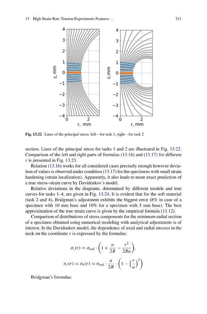
Fig. 13.22 Lines of the principal stress: left—for task 1, right—for task 2
section. Lines of the principal stress for tasks 1 and 2 are illustrated in Fig. 13.22.
Comparison of the left and right parts of formulas (13.16) and (13.17) for different
r is presented in Fig. 13.23.
Relation (13.16) works for all considered cases precisely enough however deviation of values is observed under condition (13.17) for the specimens with small strain
hardening (strain localization). Apparently, it also leads to more exact prediction of
a true stress–strain curve by Davidenkov’s model.
Relative deviations in the diagrams, determined by different models and true
curves for tasks 1–4, are given in Fig. 13.24. It is evident that for the soft material
(task 2 and 4), Bridgman’s adjustment exhibits the biggest error (8% in case of a
specimen with 10 mm base and 10% for a specimen with 5 mm base). The best
approximation of the true strain curve is given by the empirical formula (13.12).
Comparison of distributions of stress components for the minimum radial section
of a specimen obtained using numerical modeling with analytical adjustments is of
interest. In the Davidenkov model, the dependence of axial and radial stresses in the
neck on the coordinate r is expressed by the formulas:
σ z (r ) = σ real ·
1 +
a
2R
−
r
2
2Ra
,
σ r (r ) = σ θ (r ) = σ real ·
a
2R
·
1 −
r
a
2
Bridgman’s formulas:
211
Fig. 13.22 Lines of the principal stress: left—for task 1, right—for task 2
section. Lines of the principal stress for tasks 1 and 2 are illustrated in Fig. 13.22.
Comparison of the left and right parts of formulas (13.16) and (13.17) for different
r is presented in Fig. 13.23.
Relation (13.16) works for all considered cases precisely enough however deviation of values is observed under condition (13.17) for the specimens with small strain
hardening (strain localization). Apparently, it also leads to more exact prediction of
a true stress–strain curve by Davidenkov’s model.
Relative deviations in the diagrams, determined by different models and true
curves for tasks 1–4, are given in Fig. 13.24. It is evident that for the soft material
(task 2 and 4), Bridgman’s adjustment exhibits the biggest error (8% in case of a
specimen with 10 mm base and 10% for a specimen with 5 mm base). The best
approximation of the true strain curve is given by the empirical formula (13.12).
Comparison of distributions of stress components for the minimum radial section
of a specimen obtained using numerical modeling with analytical adjustments is of
interest. In the Davidenkov model, the dependence of axial and radial stresses in the
neck on the coordinate r is expressed by the formulas:
σ z (r ) = σ real ·
1 +
a
2R
−
r
2
2Ra
,
σ r (r ) = σ θ (r ) = σ real ·
a
2R
·
1 −
r
a
2
Bridgman’s formulas: