

13 High Strain Rate Tension Experiments Features …
209
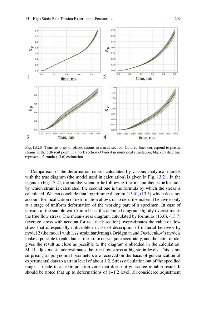
Fig. 13.20 Time histories of plastic strains in a neck section. Colored lines correspond to plastic
strains in the different point in a neck section obtained in numerical simulation; black dashed line
represents formula (13.6) estimation
Comparison of the deformation curves calculated by various analytical models
with the true diagram (the model used in calculation) is given in Fig. 13.21. In the
legend to Fig. 13.21, the numbers denote the following: the first number is the formula
by which strain is calculated, the second one is the formula by which the stress is
calculated. We can conclude that logarithmic diagram (13.4), (13.5) which does not
account for localization of deformation allows us to describe material behavior only
at a stage of uniform deformation of the working part of a specimen. In case of
tension of the sample with 5 mm base, the obtained diagram slightly overestimates
the true flow stress. The mean-stress diagram, calculated by formulas (13.6), (13.7)
(average stress with account for real neck section) overestimates the value of flow
stress that is especially noticeable in case of description of material behavior by
model 2 (the model with less strain hardening). Bridgman and Davidenkov’s models
make it possible to calculate a true strain curve quite accurately, and the latter model
gives the result as close as possible to the diagram embedded in the calculation.
MLR adjustment underestimates the true flow stress at big strain levels. This is not
surprising as polynomial parameters are received on the basis of generalization of
experimental data to a strain level of about 1.2. Stress calculation out of the specified
range is made in an extrapolation zone that does not guarantee reliable result. It
should be noted that up to deformations of 1–1.2 level, all considered adjustment
209
Fig. 13.20 Time histories of plastic strains in a neck section. Colored lines correspond to plastic
strains in the different point in a neck section obtained in numerical simulation; black dashed line
represents formula (13.6) estimation
Comparison of the deformation curves calculated by various analytical models
with the true diagram (the model used in calculation) is given in Fig. 13.21. In the
legend to Fig. 13.21, the numbers denote the following: the first number is the formula
by which strain is calculated, the second one is the formula by which the stress is
calculated. We can conclude that logarithmic diagram (13.4), (13.5) which does not
account for localization of deformation allows us to describe material behavior only
at a stage of uniform deformation of the working part of a specimen. In case of
tension of the sample with 5 mm base, the obtained diagram slightly overestimates
the true flow stress. The mean-stress diagram, calculated by formulas (13.6), (13.7)
(average stress with account for real neck section) overestimates the value of flow
stress that is especially noticeable in case of description of material behavior by
model 2 (the model with less strain hardening). Bridgman and Davidenkov’s models
make it possible to calculate a true strain curve quite accurately, and the latter model
gives the result as close as possible to the diagram embedded in the calculation.
MLR adjustment underestimates the true flow stress at big strain levels. This is not
surprising as polynomial parameters are received on the basis of generalization of
experimental data to a strain level of about 1.2. Stress calculation out of the specified
range is made in an extrapolation zone that does not guarantee reliable result. It
should be noted that up to deformations of 1–1.2 level, all considered adjustment