

13 High Strain Rate Tension Experiments Features …
203
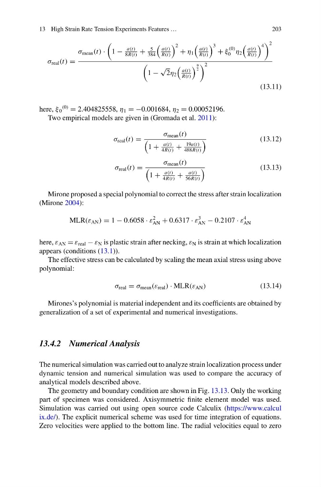
σ real (t) =
σ mean (t) ·
1 −
a(t)
8R(t)
+
5
384
a(t)
R(t)
2 + η 1
a(t)
R(t)
3 + ξ
(0)
0 η 2
a(t)
R(t)
4
2
1 −
√
2η 2
a(t)
R(t)
9
2
2
(13.11)
here, ξ 0
(0)
= 2.404825558, η 1 = −0.001684, η 2 = 0.00052196.
Two empirical models are given in (Gromada et al. 2011):
σ real (t) =
σ mean (t)
1 +
a(t)
4R(t)
+
19a(t)
488R(t)
(13.12)
σ real (t) =
σ mean (t)
1 +
a(t)
4R(t)
+
a(t)
56R(t)
(13.13)
Mirone proposed a special polynomial to correct the stress after strain localization
(Mirone 2004):
MLR(ε AN ) = 1 − 0.6058 · ε
2
AN + 0.6317 · ε
3
AN − 0.2107 · ε
4
AN
here, ε AN = ε real − ε N is plastic strain after necking, ε N is strain at which localization
appears (conditions (13.1)).
The effective stress can be calculated by scaling the mean axial stress using above
polynomial:
σ real = σ mean (ε real ) · MLR(ε AN )
(13.14)
Mirones’s polynomial is material independent and its coefficients are obtained by
generalization of a set of experimental and numerical investigations.
13.4.2 Numerical Analysis
The numerical simulation was carried out to analyze strain localization process under
dynamic tension and numerical simulation was used to compare the accuracy of
analytical models described above.
The geometry and boundary condition are shown in Fig. 13.13. Only the working
part of specimen was considered. Axisymmetric finite element model was used.
Simulation was carried out using open source code Calculix (https://www.calcul
ix.de/). The explicit numerical scheme was used for time integration of equations.
Zero velocities were applied to the bottom line. The radial velocities equal to zero
203
σ real (t) =
σ mean (t) ·
1 −
a(t)
8R(t)
+
5
384
a(t)
R(t)
2 + η 1
a(t)
R(t)
3 + ξ
(0)
0 η 2
a(t)
R(t)
4
2
1 −
√
2η 2
a(t)
R(t)
9
2
2
(13.11)
here, ξ 0
(0)
= 2.404825558, η 1 = −0.001684, η 2 = 0.00052196.
Two empirical models are given in (Gromada et al. 2011):
σ real (t) =
σ mean (t)
1 +
a(t)
4R(t)
+
19a(t)
488R(t)
(13.12)
σ real (t) =
σ mean (t)
1 +
a(t)
4R(t)
+
a(t)
56R(t)
(13.13)
Mirone proposed a special polynomial to correct the stress after strain localization
(Mirone 2004):
MLR(ε AN ) = 1 − 0.6058 · ε
2
AN + 0.6317 · ε
3
AN − 0.2107 · ε
4
AN
here, ε AN = ε real − ε N is plastic strain after necking, ε N is strain at which localization
appears (conditions (13.1)).
The effective stress can be calculated by scaling the mean axial stress using above
polynomial:
σ real = σ mean (ε real ) · MLR(ε AN )
(13.14)
Mirones’s polynomial is material independent and its coefficients are obtained by
generalization of a set of experimental and numerical investigations.
13.4.2 Numerical Analysis
The numerical simulation was carried out to analyze strain localization process under
dynamic tension and numerical simulation was used to compare the accuracy of
analytical models described above.
The geometry and boundary condition are shown in Fig. 13.13. Only the working
part of specimen was considered. Axisymmetric finite element model was used.
Simulation was carried out using open source code Calculix (https://www.calcul
ix.de/). The explicit numerical scheme was used for time integration of equations.
Zero velocities were applied to the bottom line. The radial velocities equal to zero