

13 High Strain Rate Tension Experiments Features …
201
greater plastic strain. The value of ultimate plastic strain equals to 38%. Therefore,
the large portion of stress–strain curve (almost a half) is being lost.
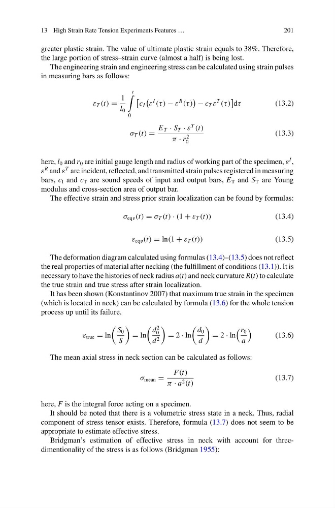
The engineering strain and engineering stress can be calculated using strain pulses
in measuring bars as follows:
ε T (t) =
1
l 0
t
0
c I
ε
I
(τ ) − ε
R
(τ )
− c T ε
T
(τ )
dτ
(13.2)
σ T (t) =
E T · S T · ε
T
(t)
π · r
2
0
(13.3)
here, l 0 and r 0 are initial gauge length and radius of working part of the specimen, ε
I ,
ε
R and ε
T are incident, reflected, and transmitted strain pulses registered in measuring
bars, c I and c T are sound speeds of input and output bars, E T and S T are Young
modulus and cross-section area of output bar.
The effective strain and stress prior strain localization can be found by formulas:
σ eqv (t) = σ T (t) · (1 + ε T (t))
(13.4)
ε eqv (t) = ln(1 + ε T (t))
(13.5)
The deformation diagram calculated using formulas (13.4)–(13.5) does not reflect
the real properties of material after necking (the fulfillment of conditions (13.1)). It is
necessary to have the histories of neck radius a(t) and neck curvature R(t) to calculate
the true strain and true stress after strain localization.
It has been shown (Konstantinov 2007) that maximum true strain in the specimen
(which is located in neck) can be calculated by formula (13.6) for the whole tension
process up until its failure.
ε true = ln
S 0
S
= ln
d
2
0
d 2
= 2 · ln
d 0
d
= 2 · ln
r 0
a
(13.6)
The mean axial stress in neck section can be calculated as follows:
σ mean =
F(t)
π · a 2 (t)
(13.7)
here, F is the integral force acting on a specimen.
It should be noted that there is a volumetric stress state in a neck. Thus, radial
component of stress tensor exists. Therefore, formula (13.7) does not seem to be
appropriate to estimate effective stress.
Bridgman’s estimation of effective stress in neck with account for threedimentionality of the stress is as follows (Bridgman 1955):
201
greater plastic strain. The value of ultimate plastic strain equals to 38%. Therefore,
the large portion of stress–strain curve (almost a half) is being lost.
The engineering strain and engineering stress can be calculated using strain pulses
in measuring bars as follows:
ε T (t) =
1
l 0
t
0
c I
ε
I
(τ ) − ε
R
(τ )
− c T ε
T
(τ )
dτ
(13.2)
σ T (t) =
E T · S T · ε
T
(t)
π · r
2
0
(13.3)
here, l 0 and r 0 are initial gauge length and radius of working part of the specimen, ε
I ,
ε
R and ε
T are incident, reflected, and transmitted strain pulses registered in measuring
bars, c I and c T are sound speeds of input and output bars, E T and S T are Young
modulus and cross-section area of output bar.
The effective strain and stress prior strain localization can be found by formulas:
σ eqv (t) = σ T (t) · (1 + ε T (t))
(13.4)
ε eqv (t) = ln(1 + ε T (t))
(13.5)
The deformation diagram calculated using formulas (13.4)–(13.5) does not reflect
the real properties of material after necking (the fulfillment of conditions (13.1)). It is
necessary to have the histories of neck radius a(t) and neck curvature R(t) to calculate
the true strain and true stress after strain localization.
It has been shown (Konstantinov 2007) that maximum true strain in the specimen
(which is located in neck) can be calculated by formula (13.6) for the whole tension
process up until its failure.
ε true = ln
S 0
S
= ln
d
2
0
d 2
= 2 · ln
d 0
d
= 2 · ln
r 0
a
(13.6)
The mean axial stress in neck section can be calculated as follows:
σ mean =
F(t)
π · a 2 (t)
(13.7)
here, F is the integral force acting on a specimen.
It should be noted that there is a volumetric stress state in a neck. Thus, radial
component of stress tensor exists. Therefore, formula (13.7) does not seem to be
appropriate to estimate effective stress.
Bridgman’s estimation of effective stress in neck with account for threedimentionality of the stress is as follows (Bridgman 1955):