

1 Modeling Fatigue Life of Structural Alloys Under Block Asymmetric Loading
5
C p = C
0
p +
t
0
˙
C p dt, ˙
χ =
2 ˙
e
p
i j ˙
e
p
i j /3
1/2 ,
χ m =
t
0
˙
χ H
F ρ
dt, χ =
t
0
˙
χ dt.
(1.5)
q χ =
q 2 Aψ 1 + (1 − A)q 1
Aψ 1 + (1 − A)
, Q s =
Q 2 Aψ 2 + (1 − A)Q 1
Aψ 2 + (1 − A)
,
a =
a 2 Aψ 3 + (1 − A)a 1
Aψ 3 + (1 − A)
, 0 ≤ ψ i ≤ 1, i = 1, 2, 3,
A = 1 − cos
2
θ, cos θ = n
e
i j n
e
i j , n
e
i j =
˙
e
i j
( ˙
e
i j ˙
e
i j ) 1/2 , n
s
i j =
S i j
(S i j S i j ) 1/2 ,
H (F ρ ) =
1, F ρ = 0 ∧ ρ i j ˙
ρ i j > 0
0, F ρ < 0 ∨ ρ i j ˙
ρ i j ≤ 0
, ,(F ρ ) = 1 − H (F ρ ),
(1.6)
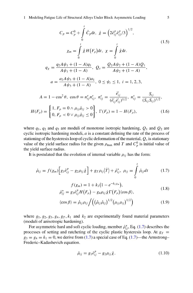
where q 1 , q 2 and q 3 are moduli of monotone isotropic hardening, Q 1 and Q 2 are
cyclic isotropic hardening moduli, a is a constant defining the rate of the process of
stationing of the hysteresis loop of cyclic deformation of the material, Q s is stationary
value of the yield surface radius for the given ρ max and T and C
0
p is initial value of
the yield surface radius.
It is postulated that the evolution of internal variable ρ i j has the form:
˙
ρ i j = f (χ m )
g 1 ˙
e
p
i j − g 2 ρ i j ˙
χ
+ g T ρ i j
˙
T
+ ˙
ρ
∗
i j , ρ i j =
t
0
˙
ρ i j dt
(1.7)
f (χ m ) = 1 + k 1
1 − e
−k 2 χ m
,
˙
ρ
∗
i j = g 3 ˙
e
p
i j H
F ρ
− g 4 ρ i j ˙
χχ
F ρ
cos β,
(1.8)
cos β = ˙
ρ i j ρ i j
˙
ρ i j ˙
ρ i j
1/2
ρ i j ρ i j
1/2
(1.9)
where g 1 , g 2 , g 3 , g 4 , g T , k 1 and k 2 are experimentally found material parameters
(moduli of anisotropic hardening).
For asymmetric hard and soft cyclic loading, member ˙
ρ
∗
i j , Eq. (1.7) describes the
processes of setting and ratcheting of the cyclic plastic hysteresis loop. At g T =
g 3 = g 4 = k 1 = 0, we derive from (1.7) a special case of Eq. (1.7)—the Armstrong–
Frederic–Kadashevich equation.
˙
ρ i j = g 1 ˙
e
p
i j − g 2 ρ i j ˙
χ.
(1.10)
5
C p = C
0
p +
t
0
˙
C p dt, ˙
χ =
2 ˙
e
p
i j ˙
e
p
i j /3
1/2 ,
χ m =
t
0
˙
χ H
F ρ
dt, χ =
t
0
˙
χ dt.
(1.5)
q χ =
q 2 Aψ 1 + (1 − A)q 1
Aψ 1 + (1 − A)
, Q s =
Q 2 Aψ 2 + (1 − A)Q 1
Aψ 2 + (1 − A)
,
a =
a 2 Aψ 3 + (1 − A)a 1
Aψ 3 + (1 − A)
, 0 ≤ ψ i ≤ 1, i = 1, 2, 3,
A = 1 − cos
2
θ, cos θ = n
e
i j n
e
i j , n
e
i j =
˙
e
i j
( ˙
e
i j ˙
e
i j ) 1/2 , n
s
i j =
S i j
(S i j S i j ) 1/2 ,
H (F ρ ) =
1, F ρ = 0 ∧ ρ i j ˙
ρ i j > 0
0, F ρ < 0 ∨ ρ i j ˙
ρ i j ≤ 0
, ,(F ρ ) = 1 − H (F ρ ),
(1.6)
where q 1 , q 2 and q 3 are moduli of monotone isotropic hardening, Q 1 and Q 2 are
cyclic isotropic hardening moduli, a is a constant defining the rate of the process of
stationing of the hysteresis loop of cyclic deformation of the material, Q s is stationary
value of the yield surface radius for the given ρ max and T and C
0
p is initial value of
the yield surface radius.
It is postulated that the evolution of internal variable ρ i j has the form:
˙
ρ i j = f (χ m )
g 1 ˙
e
p
i j − g 2 ρ i j ˙
χ
+ g T ρ i j
˙
T
+ ˙
ρ
∗
i j , ρ i j =
t
0
˙
ρ i j dt
(1.7)
f (χ m ) = 1 + k 1
1 − e
−k 2 χ m
,
˙
ρ
∗
i j = g 3 ˙
e
p
i j H
F ρ
− g 4 ρ i j ˙
χχ
F ρ
cos β,
(1.8)
cos β = ˙
ρ i j ρ i j
˙
ρ i j ˙
ρ i j
1/2
ρ i j ρ i j
1/2
(1.9)
where g 1 , g 2 , g 3 , g 4 , g T , k 1 and k 2 are experimentally found material parameters
(moduli of anisotropic hardening).
For asymmetric hard and soft cyclic loading, member ˙
ρ
∗
i j , Eq. (1.7) describes the
processes of setting and ratcheting of the cyclic plastic hysteresis loop. At g T =
g 3 = g 4 = k 1 = 0, we derive from (1.7) a special case of Eq. (1.7)—the Armstrong–
Frederic–Kadashevich equation.
˙
ρ i j = g 1 ˙
e
p
i j − g 2 ρ i j ˙
χ.
(1.10)