

166
I. P. Markov and M. V. Markina
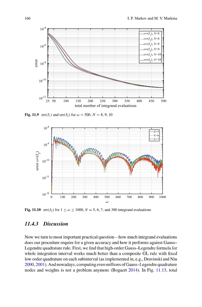
Fig. 11.9 err(I 1 ) and err(I 2 ) for ω = 500, N = 8, 9, 10
Fig. 11.10 err(I 2 ) for 1 ≤ ω ≤ 1000, N = 5, 6, 7, and 300 integrand evaluations
11.4.3 Discussion
Now we turn to most important practical question—how much integrand evaluations
does our procedure require for a given accuracy and how it performs against Gauss–
Legendre quadrature rule. First, we find that high-order Gauss–Legendre formula for
whole integration interval works much better than a composite GL rule with fixed
low order quadrature on each subinterval (as implemented in, e.g., Dravinski and Niu
2000, 2001). And nowadays, computing even millions of Gauss–Legendre quadrature
nodes and weights is not a problem anymore (Bogaert 2014). In Fig. 11.13, total
I. P. Markov and M. V. Markina
Fig. 11.9 err(I 1 ) and err(I 2 ) for ω = 500, N = 8, 9, 10
Fig. 11.10 err(I 2 ) for 1 ≤ ω ≤ 1000, N = 5, 6, 7, and 300 integrand evaluations
11.4.3 Discussion
Now we turn to most important practical question—how much integrand evaluations
does our procedure require for a given accuracy and how it performs against Gauss–
Legendre quadrature rule. First, we find that high-order Gauss–Legendre formula for
whole integration interval works much better than a composite GL rule with fixed
low order quadrature on each subinterval (as implemented in, e.g., Dravinski and Niu
2000, 2001). And nowadays, computing even millions of Gauss–Legendre quadrature
nodes and weights is not a problem anymore (Bogaert 2014). In Fig. 11.13, total