

11 Numerical Evaluation of Integrals in Laplace Domain Anisotropic …
165
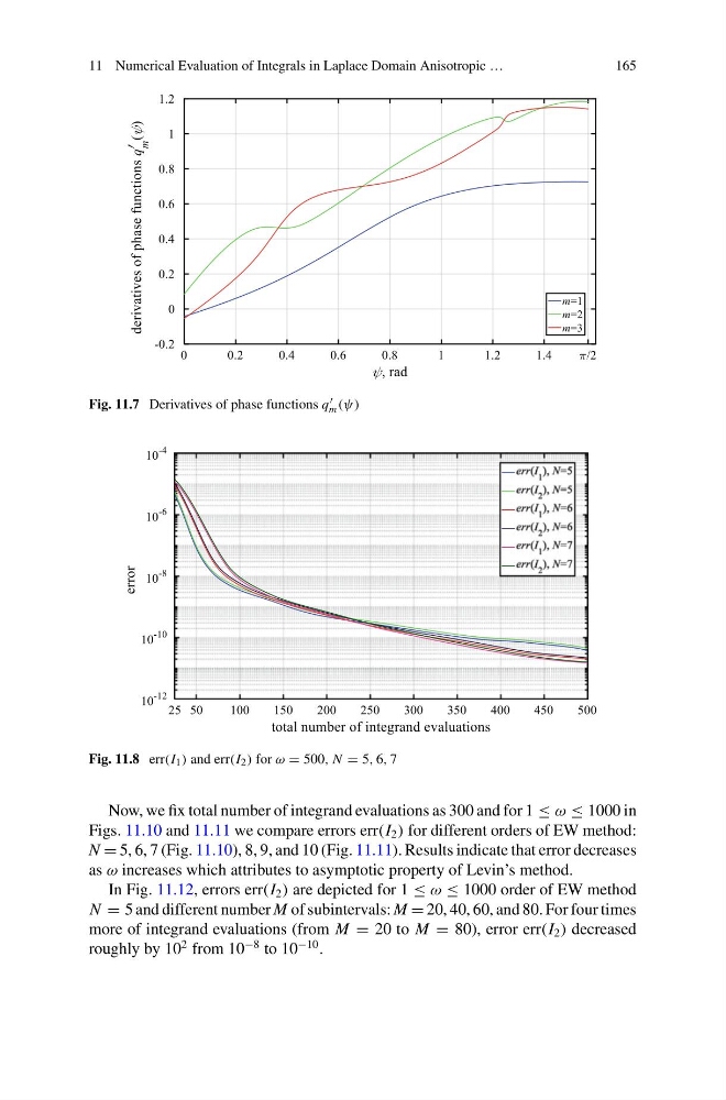
Fig. 11.7 Derivatives of phase functions q
m (ψ)
Fig. 11.8 err(I 1 ) and err(I 2 ) for ω = 500, N = 5, 6, 7
Now, we fix total number of integrand evaluations as 300 and for 1 ≤ ω ≤ 1000 in
Figs. 11.10 and 11.11 we compare errors err(I 2 ) for different orders of EW method:
N = 5, 6, 7 (Fig. 11.10), 8, 9, and 10 (Fig. 11.11). Results indicate that error decreases
as ω increases which attributes to asymptotic property of Levin’s method.
In Fig. 11.12, errors err(I 2 ) are depicted for 1 ≤ ω ≤ 1000 order of EW method
N = 5 and different number M of subintervals: M = 20, 40, 60, and 80. For four times
more of integrand evaluations (from M = 20 to M = 80), error err(I 2 ) decreased
roughly by 10
2 from 10
−8 to 10
−10 .
165
Fig. 11.7 Derivatives of phase functions q
m (ψ)
Fig. 11.8 err(I 1 ) and err(I 2 ) for ω = 500, N = 5, 6, 7
Now, we fix total number of integrand evaluations as 300 and for 1 ≤ ω ≤ 1000 in
Figs. 11.10 and 11.11 we compare errors err(I 2 ) for different orders of EW method:
N = 5, 6, 7 (Fig. 11.10), 8, 9, and 10 (Fig. 11.11). Results indicate that error decreases
as ω increases which attributes to asymptotic property of Levin’s method.
In Fig. 11.12, errors err(I 2 ) are depicted for 1 ≤ ω ≤ 1000 order of EW method
N = 5 and different number M of subintervals: M = 20, 40, 60, and 80. For four times
more of integrand evaluations (from M = 20 to M = 80), error err(I 2 ) decreased
roughly by 10
2 from 10
−8 to 10
−10 .