

162
I. P. Markov and M. V. Markina
The value of ϕ is fixed and equal π/5. The dimensionless position vectors of the
source point x and observation point y are
˜
x = [0, 0, 0]
T
,
˜
y = [sin(π/3) cos(π/4), sin(π/3) sin(π/4), cos(π/3)]
T
, ˜
r = |˜ y − ˜
x| = 1.
To measure the accuracy of the calculations, the errors are defined as
err(I 1 ) =
I
ref
1 − I 1
2
I
ref
1
2
, err(I 2 ) = max
1≤k≤3
⎛
⎝
I
i j,k;ref
2
− I
i j,k
2
2
I
i j,k;ref
2
2
⎞
⎠ ,
where 2 denotes the 2-norm (spectral norm) of a complex-valued matrix and
superscript “ref” represents converged value of I k obtained with high-order Gauss–
Legendre (GL) quadrature rule.
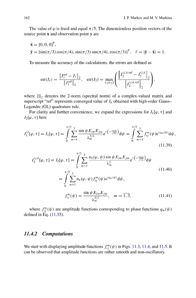
For clarity and further convenience, we expand the expressions for I 1 [ϕ, τ ] and
I 2 [ϕ, τ ] here
I
i j
1 [ϕ, τ ] = I 1 [ϕ, τ ] =
π/2
0
3
m=1
sin ψ E im E jm
λ
3/2
m
e
τ
−
cos ψ
√
λm
dψ =
π/2
0
3
m=1
f
m
i j (ψ)e
τ q m (ψ) dψ,
(11.39)
I
i j,k
2 [ϕ, τ ] = I 2 [ϕ, τ ] =
π/2
0
3
m=1
n k (ϕ, ψ) sin ψ E im E jm
λ 2
m
e
τ
−
cos ψ
√
λm
dψ
=
π/2
0
3
m=1
n k (ϕ, ψ) f
m
i j (ψ)e
τ q m (ψ) dψ,
(11.40)
f
m
i j (ψ) =
sin ψ E im E jm
λ
3/2
m
, m = 1, 3,
(11.41)
where f
m
i j (ψ) are amplitude functions corresponding to phase functions q m (ψ)
defined in Eq. (11.35).
11.4.2 Computations
We start with displaying amplitude functions f
m
i j (ψ) in Figs. 11.3, 11.4, and 11.5. It
can be observed that amplitude functions are rather smooth and non-oscillatory.
I. P. Markov and M. V. Markina
The value of ϕ is fixed and equal π/5. The dimensionless position vectors of the
source point x and observation point y are
˜
x = [0, 0, 0]
T
,
˜
y = [sin(π/3) cos(π/4), sin(π/3) sin(π/4), cos(π/3)]
T
, ˜
r = |˜ y − ˜
x| = 1.
To measure the accuracy of the calculations, the errors are defined as
err(I 1 ) =
I
ref
1 − I 1
2
I
ref
1
2
, err(I 2 ) = max
1≤k≤3
⎛
⎝
I
i j,k;ref
2
− I
i j,k
2
2
I
i j,k;ref
2
2
⎞
⎠ ,
where 2 denotes the 2-norm (spectral norm) of a complex-valued matrix and
superscript “ref” represents converged value of I k obtained with high-order Gauss–
Legendre (GL) quadrature rule.
For clarity and further convenience, we expand the expressions for I 1 [ϕ, τ ] and
I 2 [ϕ, τ ] here
I
i j
1 [ϕ, τ ] = I 1 [ϕ, τ ] =
π/2
0
3
m=1
sin ψ E im E jm
λ
3/2
m
e
τ
−
cos ψ
√
λm
dψ =
π/2
0
3
m=1
f
m
i j (ψ)e
τ q m (ψ) dψ,
(11.39)
I
i j,k
2 [ϕ, τ ] = I 2 [ϕ, τ ] =
π/2
0
3
m=1
n k (ϕ, ψ) sin ψ E im E jm
λ 2
m
e
τ
−
cos ψ
√
λm
dψ
=
π/2
0
3
m=1
n k (ϕ, ψ) f
m
i j (ψ)e
τ q m (ψ) dψ,
(11.40)
f
m
i j (ψ) =
sin ψ E im E jm
λ
3/2
m
, m = 1, 3,
(11.41)
where f
m
i j (ψ) are amplitude functions corresponding to phase functions q m (ψ)
defined in Eq. (11.35).
11.4.2 Computations
We start with displaying amplitude functions f
m
i j (ψ) in Figs. 11.3, 11.4, and 11.5. It
can be observed that amplitude functions are rather smooth and non-oscillatory.