

11 Numerical Evaluation of Integrals in Laplace Domain Anisotropic …
161
β(ϕ, ψ) = d(ϕ) cos ψ − e sin ψ = [β 1 , β 2 , β 3 ]
T
,
(11.37)
jk (n, β) = C i jkl (β i n l + n i β l ), i, j, k, l = 1, 3,
(11.38)
where it should be noted that there is no summation in Eq. (11.36) over m.
We propose the following simple procedure for computing integrals I 1 [ϕ, τ ] and
I 2 [ϕ, τ ].
1. Subdivide an integration interval [0, π/2] into sufficient number of subintervals.
Perform integration with Evans-Webster quadrature rule on each subinterval and
then sum all partial results.
2. We assume that for a relatively large number of subintervals, phase function
may contain only one stationary point in each subinterval. Hence, to determine
if phase function has stationary point in a current subinterval, we simply have to
check the signs of the phase function derivative at the end points of subinterval. If
signs are different, then the phase function has stationary point in the subinterval.
3. If there is a stationary point in the current subinterval, a complex-valued linear
algebraic system for weights w j (11.31) becomes ill-conditioned or even singular.
In order to deal with such system, we use truncated singular value decomposition.
11.4 Numerical Example and Discussions
11.4.1 Numerical Example Explanation
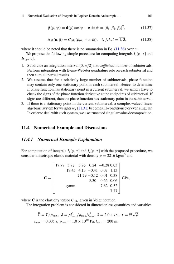
For computation of integrals I 1 [ϕ, τ ] and I 2 [ϕ, τ ] with the proposed procedure, we
consider anisotropic elastic material with density ρ = 2216 kg/m
3 and
C =
⎡
⎢
⎢
⎢
⎢
⎢
⎢
⎢
⎣
17.77 3.78 3.76 0.24 −0.28 0.03
19.45 4.13 −0.41 0.07 1.13
21.79 −0.12 0.01 0.38
8.30 0.66 0.06
symm.
7.62 0.52
7.77
⎤
⎥
⎥
⎥
⎥
⎥
⎥
⎥
⎦
GPa,
where C is the elasticity tensor C i jkl given in Voigt notation.
The integration problem is considered in dimensionless quantities and variables
C = C/ p max , ˜
ρ = ρl
2
max / p max /t
2
max , ˜
s = 2.0 + iω, τ = ˜
s ˜
r
˜
ρ,
t max = 0.005 s, p max = 1.0 × 10
10 Pa, l max = 200 m.
161
β(ϕ, ψ) = d(ϕ) cos ψ − e sin ψ = [β 1 , β 2 , β 3 ]
T
,
(11.37)
jk (n, β) = C i jkl (β i n l + n i β l ), i, j, k, l = 1, 3,
(11.38)
where it should be noted that there is no summation in Eq. (11.36) over m.
We propose the following simple procedure for computing integrals I 1 [ϕ, τ ] and
I 2 [ϕ, τ ].
1. Subdivide an integration interval [0, π/2] into sufficient number of subintervals.
Perform integration with Evans-Webster quadrature rule on each subinterval and
then sum all partial results.
2. We assume that for a relatively large number of subintervals, phase function
may contain only one stationary point in each subinterval. Hence, to determine
if phase function has stationary point in a current subinterval, we simply have to
check the signs of the phase function derivative at the end points of subinterval. If
signs are different, then the phase function has stationary point in the subinterval.
3. If there is a stationary point in the current subinterval, a complex-valued linear
algebraic system for weights w j (11.31) becomes ill-conditioned or even singular.
In order to deal with such system, we use truncated singular value decomposition.
11.4 Numerical Example and Discussions
11.4.1 Numerical Example Explanation
For computation of integrals I 1 [ϕ, τ ] and I 2 [ϕ, τ ] with the proposed procedure, we
consider anisotropic elastic material with density ρ = 2216 kg/m
3 and
C =
⎡
⎢
⎢
⎢
⎢
⎢
⎢
⎢
⎣
17.77 3.78 3.76 0.24 −0.28 0.03
19.45 4.13 −0.41 0.07 1.13
21.79 −0.12 0.01 0.38
8.30 0.66 0.06
symm.
7.62 0.52
7.77
⎤
⎥
⎥
⎥
⎥
⎥
⎥
⎥
⎦
GPa,
where C is the elasticity tensor C i jkl given in Voigt notation.
The integration problem is considered in dimensionless quantities and variables
C = C/ p max , ˜
ρ = ρl
2
max / p max /t
2
max , ˜
s = 2.0 + iω, τ = ˜
s ˜
r
˜
ρ,
t max = 0.005 s, p max = 1.0 × 10
10 Pa, l max = 200 m.