

158
I. P. Markov and M. V. Markina
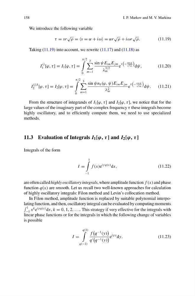
We introduce the following variable
τ = sr
√
ρ = s = α + iω = αr
√
ρ + iωr
√ ρ.
(11.19)
Taking (11.19) into account, we rewrite (11.17) and (11.18) as
I
i j
1 [ϕ, τ ] = I 1 [ϕ, τ ] =
π/2
0
3
m=1
sin ψ E im E jm
λ
3/2
m
e
τ
−
cos ψ
√
λm
dψ,
(11.20)
I
i j,k
2 [ϕ, τ ] = I 2 [ϕ, τ ] =
π/2
0
3
m=1
sin ψn k (ϕ, ψ)E im E jm
λ 2
m
e
τ
−
cos ψ
√ λm
dψ.
(11.21)
From the structure of integrands of I 1 [ϕ, τ ] and I 2 [ϕ, τ ], we notice that for the
large values of the imaginary part of the complex frequency τ these integrals become
highly oscillatory, and to efficiently compute them, we need to use specialized
methods.
11.3 Evaluation of Integrals I 1 [ϕ, τ ] and I 2 [ϕ, τ ]
Integrals of the form
I =
1
−1
f (x)e
iγ q(x) dx,
(11.22)
are often called highly oscillatory integrals, where amplitude function f (x) and phase
function q(x) are smooth. Let us recall two well-known approaches for calculation
of highly oscillatory integrals: Filon method and Levin’s collocation method.
In Filon method, amplitude function is replaced by suitable polynomial interpolating function, and then, oscillatory integral can be evaluated by computing moments
1
−1 x
k e
iγ q(x) dx, k = 0, 1, 2, . . .. This strategy if very effective for the integrals with
linear phase functions or for the integrals in which the following change of variables
is possible
I =
q(1)
q(−1)
f
q
−1
(y)
q
q −1 (y)
e
iγ y dy.
(11.23)
I. P. Markov and M. V. Markina
We introduce the following variable
τ = sr
√
ρ = s = α + iω = αr
√
ρ + iωr
√ ρ.
(11.19)
Taking (11.19) into account, we rewrite (11.17) and (11.18) as
I
i j
1 [ϕ, τ ] = I 1 [ϕ, τ ] =
π/2
0
3
m=1
sin ψ E im E jm
λ
3/2
m
e
τ
−
cos ψ
√
λm
dψ,
(11.20)
I
i j,k
2 [ϕ, τ ] = I 2 [ϕ, τ ] =
π/2
0
3
m=1
sin ψn k (ϕ, ψ)E im E jm
λ 2
m
e
τ
−
cos ψ
√ λm
dψ.
(11.21)
From the structure of integrands of I 1 [ϕ, τ ] and I 2 [ϕ, τ ], we notice that for the
large values of the imaginary part of the complex frequency τ these integrals become
highly oscillatory, and to efficiently compute them, we need to use specialized
methods.
11.3 Evaluation of Integrals I 1 [ϕ, τ ] and I 2 [ϕ, τ ]
Integrals of the form
I =
1
−1
f (x)e
iγ q(x) dx,
(11.22)
are often called highly oscillatory integrals, where amplitude function f (x) and phase
function q(x) are smooth. Let us recall two well-known approaches for calculation
of highly oscillatory integrals: Filon method and Levin’s collocation method.
In Filon method, amplitude function is replaced by suitable polynomial interpolating function, and then, oscillatory integral can be evaluated by computing moments
1
−1 x
k e
iγ q(x) dx, k = 0, 1, 2, . . .. This strategy if very effective for the integrals with
linear phase functions or for the integrals in which the following change of variables
is possible
I =
q(1)
q(−1)
f
q
−1
(y)
q
q −1 (y)
e
iγ y dy.
(11.23)