

11 Numerical Evaluation of Integrals in Laplace Domain Anisotropic …
157
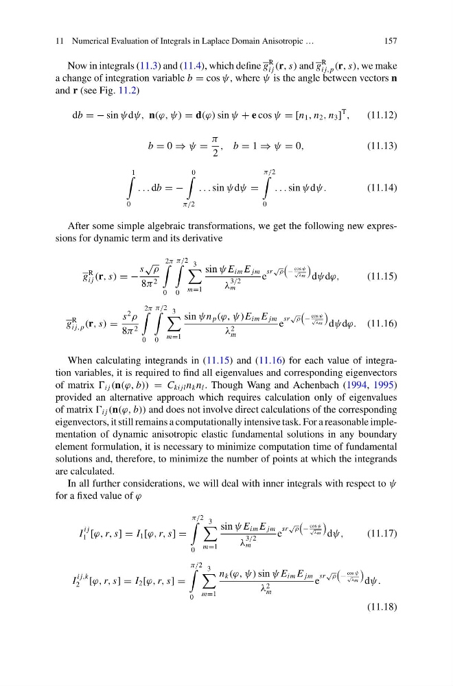
Now in integrals (11.3) and (11.4), which define g
R
i j (r, s) and g
R
i j, p (r, s), we make
a change of integration variable b = cos ψ, where ψ is the angle between vectors n
and r (see Fig. 11.2)
db = − sin ψdψ, n(ϕ, ψ) = d(ϕ) sin ψ + e cos ψ = [n 1 , n 2 , n 3 ]
T
,
(11.12)
b = 0 ⇒ ψ =
π
2
, b = 1 ⇒ ψ = 0,
(11.13)
1
0
. . . db = −
0
π/2
. . . sin ψdψ =
π/2
0
. . . sin ψdψ.
(11.14)
After some simple algebraic transformations, we get the following new expressions for dynamic term and its derivative
g
R
i j (r, s) = −
s
√ ρ
8π 2
2π
0
π/2
0
3
m=1
sin ψ E im E jm
λ
3/2
m
e
sr
√ ρ
−
cos ψ
√ λm
dψdϕ,
(11.15)
g
R
i j, p (r, s) =
s
2
ρ
8π 2
2π
0
π/2
0
3
m=1
sin ψn p (ϕ, ψ)E im E jm
λ 2
m
e
sr
√ ρ
−
cos ψ
√
λm
dψdϕ. (11.16)
When calculating integrands in (11.15) and (11.16) for each value of integration variables, it is required to find all eigenvalues and corresponding eigenvectors
of matrix i j (n(ϕ, b)) = C ki jl n k n l . Though Wang and Achenbach (1994, 1995)
provided an alternative approach which requires calculation only of eigenvalues
of matrix i j (n(ϕ, b)) and does not involve direct calculations of the corresponding
eigenvectors, it still remains a computationally intensive task. For a reasonable implementation of dynamic anisotropic elastic fundamental solutions in any boundary
element formulation, it is necessary to minimize computation time of fundamental
solutions and, therefore, to minimize the number of points at which the integrands
are calculated.
In all further considerations, we will deal with inner integrals with respect to ψ
for a fixed value of ϕ
I
i j
1 [ϕ, r, s] = I 1 [ϕ, r, s] =
π/2
0
3
m=1
sin ψ E im E jm
λ
3/2
m
e
sr
√ ρ
−
cos ψ
√ λm
dψ,
(11.17)
I
i j,k
2 [ϕ, r, s] = I 2 [ϕ, r, s] =
π/2
0
3
m=1
n k (ϕ, ψ) sin ψ E im E jm
λ 2
m
e
sr
√ ρ
−
cos ψ
√ λm
dψ.
(11.18)
157
Now in integrals (11.3) and (11.4), which define g
R
i j (r, s) and g
R
i j, p (r, s), we make
a change of integration variable b = cos ψ, where ψ is the angle between vectors n
and r (see Fig. 11.2)
db = − sin ψdψ, n(ϕ, ψ) = d(ϕ) sin ψ + e cos ψ = [n 1 , n 2 , n 3 ]
T
,
(11.12)
b = 0 ⇒ ψ =
π
2
, b = 1 ⇒ ψ = 0,
(11.13)
1
0
. . . db = −
0
π/2
. . . sin ψdψ =
π/2
0
. . . sin ψdψ.
(11.14)
After some simple algebraic transformations, we get the following new expressions for dynamic term and its derivative
g
R
i j (r, s) = −
s
√ ρ
8π 2
2π
0
π/2
0
3
m=1
sin ψ E im E jm
λ
3/2
m
e
sr
√ ρ
−
cos ψ
√ λm
dψdϕ,
(11.15)
g
R
i j, p (r, s) =
s
2
ρ
8π 2
2π
0
π/2
0
3
m=1
sin ψn p (ϕ, ψ)E im E jm
λ 2
m
e
sr
√ ρ
−
cos ψ
√
λm
dψdϕ. (11.16)
When calculating integrands in (11.15) and (11.16) for each value of integration variables, it is required to find all eigenvalues and corresponding eigenvectors
of matrix i j (n(ϕ, b)) = C ki jl n k n l . Though Wang and Achenbach (1994, 1995)
provided an alternative approach which requires calculation only of eigenvalues
of matrix i j (n(ϕ, b)) and does not involve direct calculations of the corresponding
eigenvectors, it still remains a computationally intensive task. For a reasonable implementation of dynamic anisotropic elastic fundamental solutions in any boundary
element formulation, it is necessary to minimize computation time of fundamental
solutions and, therefore, to minimize the number of points at which the integrands
are calculated.
In all further considerations, we will deal with inner integrals with respect to ψ
for a fixed value of ϕ
I
i j
1 [ϕ, r, s] = I 1 [ϕ, r, s] =
π/2
0
3
m=1
sin ψ E im E jm
λ
3/2
m
e
sr
√ ρ
−
cos ψ
√ λm
dψ,
(11.17)
I
i j,k
2 [ϕ, r, s] = I 2 [ϕ, r, s] =
π/2
0
3
m=1
n k (ϕ, ψ) sin ψ E im E jm
λ 2
m
e
sr
√ ρ
−
cos ψ
√ λm
dψ.
(11.18)