

146
G. Yu. Levi et al.
l
(n)
1k = −iα(c
∗(n)
3113 σ
(n)
k f
(n)
1k + c
∗(n)
1313 f
(n)
3k ),
l
(n)
3k = −α
2 c
∗(n)
1133 f
(n)
1k + σ
(n)
k c
∗(n)
3333 f
(n)
3k − β
∗(n)
3
f
(n)
4k ,
l
(n)
4k = σ
(n)
k f 4k , u
(n)
p s
(n)
k = f
(n)
pk sh(−hσ
(n)
k ), u
(n)
p c
(n)
k = f
(n)
pk ch(−hσ
(n)
k ),
u
(n)
p e
(n)
k = f
(n)
pk e
(−hσ
(n)
k )
, c
(1)
k = ch(−hσ
(1)
k ),
s
(1)
k = sh(−hσ
(1)
k ), e
(0)
k = e
(−hσ
(0)
k )
.
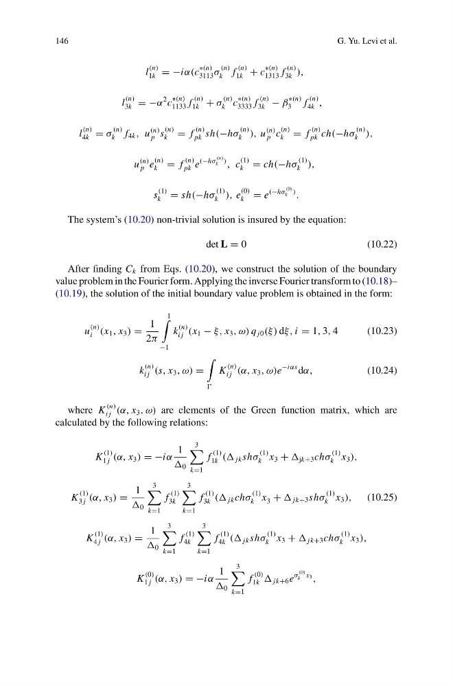
The system’s (10.20) non-trivial solution is insured by the equation:
det L = 0
(10.22)
After finding C k from Eqs. (10.20), we construct the solution of the boundary
value problem in the Fourier form. Applying the inverse Fourier transform to (10.18)–
(10.19), the solution of the initial boundary value problem is obtained in the form:
u
(n)
i (x 1 , x 3 ) =
1
2π
1
−1
k
(n)
i j (x 1 − ξ, x 3 , ω) q j0 (ξ ) dξ, i = 1, 3, 4
(10.23)
k
(n)
i j (s, x 3 , ω) =
K
(n)
i j (α, x 3 , ω)e
−iαs dα,
(10.24)
where K
(n)
i j (α, x 3 , ω) are elements of the Green function matrix, which are
calculated by the following relations:
K
(1)
1 j (α, x 3 ) = −iα
1
0
3
k=1
f
(1)
1k (( jk shσ
(1)
k x 3 + jk+3 chσ
(1)
k x 3 ),
K
(1)
3 j (α, x 3 ) =
1
0
3
k=1
f
(1)
3k
3
k=1
f
(1)
3k (( jk chσ
(1)
k x 3 + jk+3 shσ
(1)
k x 3 ), (10.25)
K
(1)
4 j (α, x 3 ) =
1
0
3
k=1
f
(1)
4k
3
k=1
f
(1)
4k (( jk shσ
(1)
k x 3 + jk+3 chσ
(1)
k x 3 ),
K
(0)
1 j (α, x 3 ) = −iα
1
0
3
k=1
f
(0)
1k jk+6 e
σ
(0)
k x 3 ,
G. Yu. Levi et al.
l
(n)
1k = −iα(c
∗(n)
3113 σ
(n)
k f
(n)
1k + c
∗(n)
1313 f
(n)
3k ),
l
(n)
3k = −α
2 c
∗(n)
1133 f
(n)
1k + σ
(n)
k c
∗(n)
3333 f
(n)
3k − β
∗(n)
3
f
(n)
4k ,
l
(n)
4k = σ
(n)
k f 4k , u
(n)
p s
(n)
k = f
(n)
pk sh(−hσ
(n)
k ), u
(n)
p c
(n)
k = f
(n)
pk ch(−hσ
(n)
k ),
u
(n)
p e
(n)
k = f
(n)
pk e
(−hσ
(n)
k )
, c
(1)
k = ch(−hσ
(1)
k ),
s
(1)
k = sh(−hσ
(1)
k ), e
(0)
k = e
(−hσ
(0)
k )
.
The system’s (10.20) non-trivial solution is insured by the equation:
det L = 0
(10.22)
After finding C k from Eqs. (10.20), we construct the solution of the boundary
value problem in the Fourier form. Applying the inverse Fourier transform to (10.18)–
(10.19), the solution of the initial boundary value problem is obtained in the form:
u
(n)
i (x 1 , x 3 ) =
1
2π
1
−1
k
(n)
i j (x 1 − ξ, x 3 , ω) q j0 (ξ ) dξ, i = 1, 3, 4
(10.23)
k
(n)
i j (s, x 3 , ω) =
K
(n)
i j (α, x 3 , ω)e
−iαs dα,
(10.24)
where K
(n)
i j (α, x 3 , ω) are elements of the Green function matrix, which are
calculated by the following relations:
K
(1)
1 j (α, x 3 ) = −iα
1
0
3
k=1
f
(1)
1k (( jk shσ
(1)
k x 3 + jk+3 chσ
(1)
k x 3 ),
K
(1)
3 j (α, x 3 ) =
1
0
3
k=1
f
(1)
3k
3
k=1
f
(1)
3k (( jk chσ
(1)
k x 3 + jk+3 shσ
(1)
k x 3 ), (10.25)
K
(1)
4 j (α, x 3 ) =
1
0
3
k=1
f
(1)
4k
3
k=1
f
(1)
4k (( jk shσ
(1)
k x 3 + jk+3 chσ
(1)
k x 3 ),
K
(0)
1 j (α, x 3 ) = −iα
1
0
3
k=1
f
(0)
1k jk+6 e
σ
(0)
k x 3 ,