

159
ranking: indices on Charts
The next step is to seek, from the subset of materials that meet the
property limits, those that maximize the performance of the component. We use the design of light, stiff components as examples;
the other material indices are used in a similar way.
Figure 5.10 shows a schematic of the E − ρ chart shown earlier.
The logarithmic scales allow all three of the indices E/ρ, E
1/3
/ρ, and
E
1/2 /ρ, listed in Table A.2 in the Appendix, to be plotted onto it.
Consider the condition
M
E cons
t C
= =
ρ
tan ,
(5.1)
that is, a particular value of the specific stiffness. Taking logs
log
log
log
E
C
( ) = ( ) + ( )
ρ
(5.2)
This is the equation of a straight line of slope 1 on a plot of log(E)
against log(ρ), as shown on the figure. Similarly, the condition
M
E
cons
t C
=
=
1 3
ρ
tan ,
(5.3)
becomes, on taking logs,
log
log
log
E
C
( ) =
( ) +
( )
3
3
ρ
(5.4)
This is another straight line, this time with a slope of 3, also shown.
And by inspection, the third index E
1/2
/ρ will plot as a line of slope
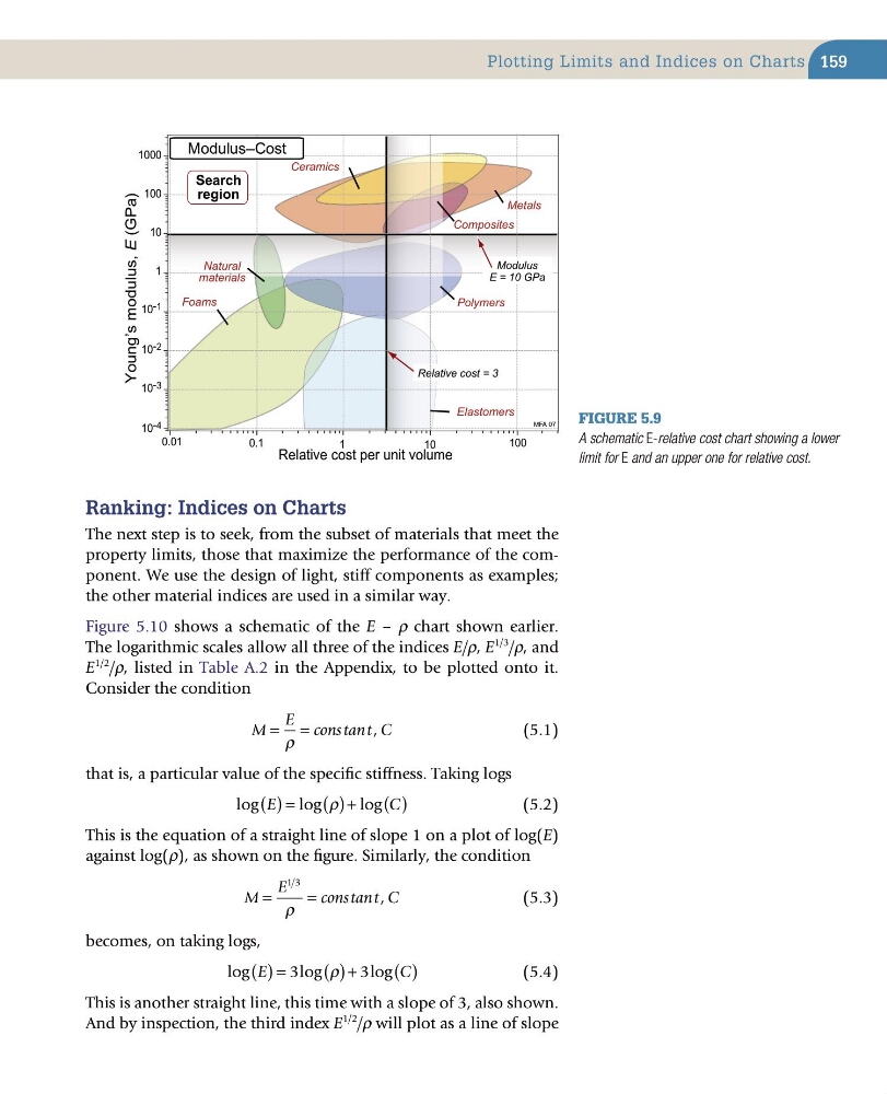
Figure 5.9
A schematic E-relative cost chart showing a lower
limit for E and an upper one for relative cost.
Relative cost = 3
Relative cost per unit volume
Young’s modulus, E (GPa)
10 -4
10 -3
10 -2
10 -1
1
10
100
1000
Metals
Polymers
Natural
materials
Composites
Foams
Ceramics
Elastomers
Modulus–Cost
MFA 07
0.01
0.1
1
10
100
Modulus
E = 10 GPa
Search
region
Plotting Limits and Indices on Charts
ranking: indices on Charts
The next step is to seek, from the subset of materials that meet the
property limits, those that maximize the performance of the component. We use the design of light, stiff components as examples;
the other material indices are used in a similar way.
Figure 5.10 shows a schematic of the E − ρ chart shown earlier.
The logarithmic scales allow all three of the indices E/ρ, E
1/3
/ρ, and
E
1/2 /ρ, listed in Table A.2 in the Appendix, to be plotted onto it.
Consider the condition
M
E cons
t C
= =
ρ
tan ,
(5.1)
that is, a particular value of the specific stiffness. Taking logs
log
log
log
E
C
( ) = ( ) + ( )
ρ
(5.2)
This is the equation of a straight line of slope 1 on a plot of log(E)
against log(ρ), as shown on the figure. Similarly, the condition
M
E
cons
t C
=
=
1 3
ρ
tan ,
(5.3)
becomes, on taking logs,
log
log
log
E
C
( ) =
( ) +
( )
3
3
ρ
(5.4)
This is another straight line, this time with a slope of 3, also shown.
And by inspection, the third index E
1/2
/ρ will plot as a line of slope
Figure 5.9
A schematic E-relative cost chart showing a lower
limit for E and an upper one for relative cost.
Relative cost = 3
Relative cost per unit volume
Young’s modulus, E (GPa)
10 -4
10 -3
10 -2
10 -1
1
10
100
1000
Metals
Polymers
Natural
materials
Composites
Foams
Ceramics
Elastomers
Modulus–Cost
MFA 07
0.01
0.1
1
10
100
Modulus
E = 10 GPa
Search
region
Plotting Limits and Indices on Charts