

74
5 Quantum Key Distribution with Imperfect Devices
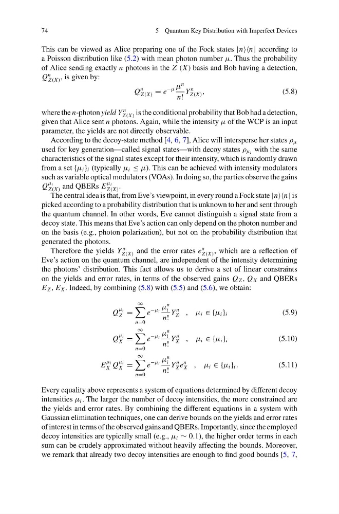
This can be viewed as Alice preparing one of the Fock states |nn | according to
a Poisson distribution like (5.2) with mean photon number μ. Thus the probability
of Alice sending exactly n photons in the Z (X ) basis and Bob having a detection,
Q
n
Z (X ) , is given by:
Q
n
Z (X ) = e
−μ μ
n
n!
Y
n
Z (X ) ,
(5.8)
where the n-photon yield Y
n
Z (X ) is the conditional probability that Bob had a detection,
given that Alice sent n photons. Again, while the intensity μ of the WCP is an input
parameter, the yields are not directly observable.
According to the decoy-state method [4, 6, 7], Alice will intersperse her states ρ μ
used for key generation—called signal states—with decoy states ρ μ i with the same
characteristics of the signal states except for their intensity, which is randomly drawn
from a set {μ i } i (typically μ i ≤ μ). This can be achieved with intensity modulators
such as variable optical modulators (VOAs). In doing so, the parties observe the gains
Q
μ i
Z (X ) and QBERs E
μ i
Z (X ) .
The central idea is that, from Eve’s viewpoint, in every round a Fock state |nn | is
picked according to a probability distribution that is unknown to her and sent through
the quantum channel. In other words, Eve cannot distinguish a signal state from a
decoy state. This means that Eve’s action can only depend on the photon number and
on the basis (e.g., photon polarization), but not on the probability distribution that
generated the photons.
Therefore the yields Y
n
Z (X ) and the error rates e
n
Z (X ) , which are a reflection of
Eve’s action on the quantum channel, are independent of the intensity determining
the photons’ distribution. This fact allows us to derive a set of linear constraints
on the yields and error rates, in terms of the observed gains Q Z , Q X and QBERs
E Z , E X . Indeed, by combining (5.8) with (5.5) and (5.6), we obtain:
Q
μ i
Z =
∞
n=0
e
−μ i
μ
n
i
n!
Y
n
Z , μ i ∈ {μ i } i
(5.9)
Q
μ i
X =
∞
n=0
e
−μ i
μ
n
i
n!
Y
n
X , μ i ∈ {μ i } i
(5.10)
E
μ i
X Q
μ i
X =
∞
n=0
e
−μ i
μ
n
i
n!
Y
n
X e
n
X , μ i ∈ {μ i } i .
(5.11)
Every equality above represents a system of equations determined by different decoy
intensities μ i . The larger the number of decoy intensities, the more constrained are
the yields and error rates. By combining the different equations in a system with
Gaussian elimination techniques, one can derive bounds on the yields and error rates
of interest in terms of the observed gains and QBERs. Importantly, since the employed
decoy intensities are typically small (e.g., μ i ∼ 0.1), the higher order terms in each
sum can be crudely approximated without heavily affecting the bounds. Moreover,
we remark that already two decoy intensities are enough to find good bounds [5, 7,
5 Quantum Key Distribution with Imperfect Devices
This can be viewed as Alice preparing one of the Fock states |nn | according to
a Poisson distribution like (5.2) with mean photon number μ. Thus the probability
of Alice sending exactly n photons in the Z (X ) basis and Bob having a detection,
Q
n
Z (X ) , is given by:
Q
n
Z (X ) = e
−μ μ
n
n!
Y
n
Z (X ) ,
(5.8)
where the n-photon yield Y
n
Z (X ) is the conditional probability that Bob had a detection,
given that Alice sent n photons. Again, while the intensity μ of the WCP is an input
parameter, the yields are not directly observable.
According to the decoy-state method [4, 6, 7], Alice will intersperse her states ρ μ
used for key generation—called signal states—with decoy states ρ μ i with the same
characteristics of the signal states except for their intensity, which is randomly drawn
from a set {μ i } i (typically μ i ≤ μ). This can be achieved with intensity modulators
such as variable optical modulators (VOAs). In doing so, the parties observe the gains
Q
μ i
Z (X ) and QBERs E
μ i
Z (X ) .
The central idea is that, from Eve’s viewpoint, in every round a Fock state |nn | is
picked according to a probability distribution that is unknown to her and sent through
the quantum channel. In other words, Eve cannot distinguish a signal state from a
decoy state. This means that Eve’s action can only depend on the photon number and
on the basis (e.g., photon polarization), but not on the probability distribution that
generated the photons.
Therefore the yields Y
n
Z (X ) and the error rates e
n
Z (X ) , which are a reflection of
Eve’s action on the quantum channel, are independent of the intensity determining
the photons’ distribution. This fact allows us to derive a set of linear constraints
on the yields and error rates, in terms of the observed gains Q Z , Q X and QBERs
E Z , E X . Indeed, by combining (5.8) with (5.5) and (5.6), we obtain:
Q
μ i
Z =
∞
n=0
e
−μ i
μ
n
i
n!
Y
n
Z , μ i ∈ {μ i } i
(5.9)
Q
μ i
X =
∞
n=0
e
−μ i
μ
n
i
n!
Y
n
X , μ i ∈ {μ i } i
(5.10)
E
μ i
X Q
μ i
X =
∞
n=0
e
−μ i
μ
n
i
n!
Y
n
X e
n
X , μ i ∈ {μ i } i .
(5.11)
Every equality above represents a system of equations determined by different decoy
intensities μ i . The larger the number of decoy intensities, the more constrained are
the yields and error rates. By combining the different equations in a system with
Gaussian elimination techniques, one can derive bounds on the yields and error rates
of interest in terms of the observed gains and QBERs. Importantly, since the employed
decoy intensities are typically small (e.g., μ i ∼ 0.1), the higher order terms in each
sum can be crudely approximated without heavily affecting the bounds. Moreover,
we remark that already two decoy intensities are enough to find good bounds [5, 7,