

7.5 Conditional Entropy Bound
121
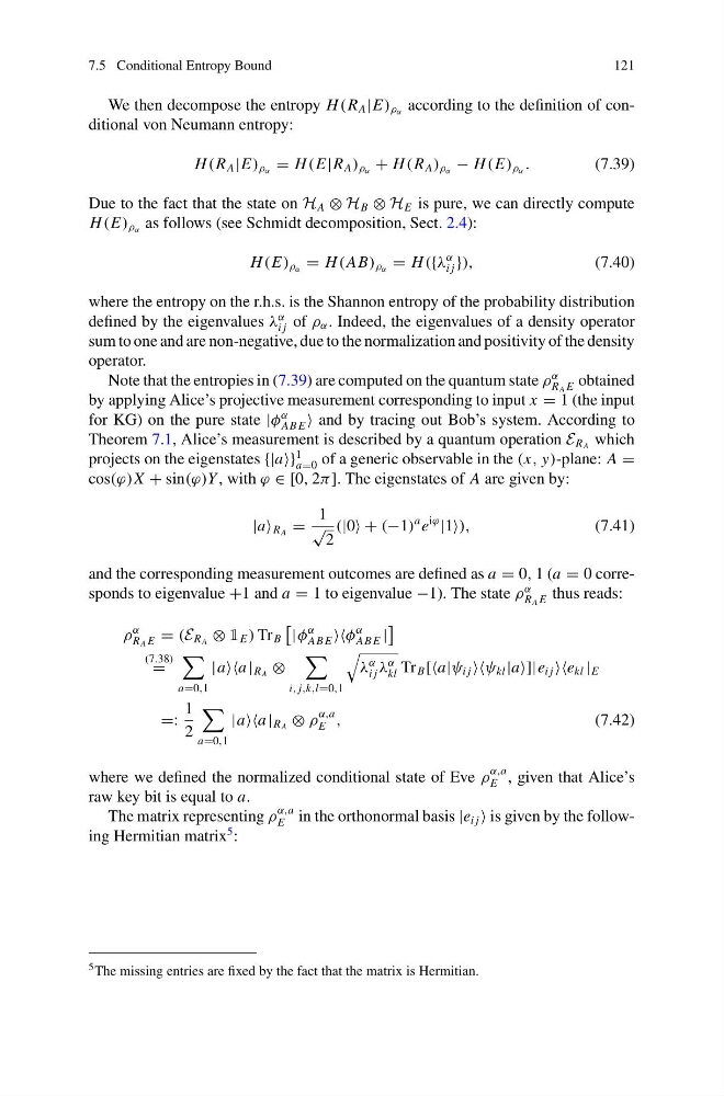
We then decompose the entropy H (R A |E) ρ α according to the definition of conditional von Neumann entropy:
H (R A |E) ρ α = H (E|R A ) ρ α + H (R A ) ρ α − H (E) ρ α .
(7.39)
Due to the fact that the state on H A ⊗ H B ⊗ H E is pure, we can directly compute
H (E) ρ α as follows (see Schmidt decomposition, Sect. 2.4):
H (E) ρ α = H (AB) ρ α = H ({λ
α
i j }),
(7.40)
where the entropy on the r.h.s. is the Shannon entropy of the probability distribution
defined by the eigenvalues λ
α
i j of ρ α . Indeed, the eigenvalues of a density operator
sum to one and are non-negative, due to the normalization and positivity of the density
operator.
Note that the entropies in (7.39) are computed on the quantum state ρ
α
R A E obtained
by applying Alice’s projective measurement corresponding to input x = 1 (the input
for KG) on the pure state |φ
α
AB E and by tracing out Bob’s system. According to
Theorem 7.1, Alice’s measurement is described by a quantum operation E R A which
projects on the eigenstates {|a}
1
a=0 of a generic observable in the (x, y)-plane: A =
cos(ϕ)X + sin(ϕ)Y , with ϕ ∈ [0, 2π ]. The eigenstates of A are given by:
|a R A =
1
√
2
(|0 + (−1)
a e
iϕ
|1),
(7.41)
and the corresponding measurement outcomes are defined as a = 0, 1 (a = 0 corresponds to eigenvalue +1 and a = 1 to eigenvalue −1). The state ρ
α
R A E thus reads:
ρ
α
R A E = (E R A ⊗ 1 E ) Tr B
|φ
α
AB E φ
α
AB E |
(7.38)
=
a=0,1
|aa | R A ⊗
i, j,k,l=0,1
λ
α
i j λ
α
kl Tr B [[a|ψ i j ψ kl |a]|e i j e kl | E
=:
1
2
a=0,1
|aa | R A ⊗ ρ
α,a
E ,
(7.42)
where we defined the normalized conditional state of Eve ρ
α,a
E , given that Alice’s
raw key bit is equal to a.
The matrix representing ρ
α,a
E in the orthonormal basis |e i j is given by the following Hermitian matrix
5 :
5 The missing entries are fixed by the fact that the matrix is Hermitian.
121
We then decompose the entropy H (R A |E) ρ α according to the definition of conditional von Neumann entropy:
H (R A |E) ρ α = H (E|R A ) ρ α + H (R A ) ρ α − H (E) ρ α .
(7.39)
Due to the fact that the state on H A ⊗ H B ⊗ H E is pure, we can directly compute
H (E) ρ α as follows (see Schmidt decomposition, Sect. 2.4):
H (E) ρ α = H (AB) ρ α = H ({λ
α
i j }),
(7.40)
where the entropy on the r.h.s. is the Shannon entropy of the probability distribution
defined by the eigenvalues λ
α
i j of ρ α . Indeed, the eigenvalues of a density operator
sum to one and are non-negative, due to the normalization and positivity of the density
operator.
Note that the entropies in (7.39) are computed on the quantum state ρ
α
R A E obtained
by applying Alice’s projective measurement corresponding to input x = 1 (the input
for KG) on the pure state |φ
α
AB E and by tracing out Bob’s system. According to
Theorem 7.1, Alice’s measurement is described by a quantum operation E R A which
projects on the eigenstates {|a}
1
a=0 of a generic observable in the (x, y)-plane: A =
cos(ϕ)X + sin(ϕ)Y , with ϕ ∈ [0, 2π ]. The eigenstates of A are given by:
|a R A =
1
√
2
(|0 + (−1)
a e
iϕ
|1),
(7.41)
and the corresponding measurement outcomes are defined as a = 0, 1 (a = 0 corresponds to eigenvalue +1 and a = 1 to eigenvalue −1). The state ρ
α
R A E thus reads:
ρ
α
R A E = (E R A ⊗ 1 E ) Tr B
|φ
α
AB E φ
α
AB E |
(7.38)
=
a=0,1
|aa | R A ⊗
i, j,k,l=0,1
λ
α
i j λ
α
kl Tr B [[a|ψ i j ψ kl |a]|e i j e kl | E
=:
1
2
a=0,1
|aa | R A ⊗ ρ
α,a
E ,
(7.42)
where we defined the normalized conditional state of Eve ρ
α,a
E , given that Alice’s
raw key bit is equal to a.
The matrix representing ρ
α,a
E in the orthonormal basis |e i j is given by the following Hermitian matrix
5 :
5 The missing entries are fixed by the fact that the matrix is Hermitian.