

7.1 Bell’s Theorem
109
S CHSH = =a 0 b 0 + +a 0 b 1 + +a 1 b 0 − −a 1 b 1 ≤ 2.
(7.9)
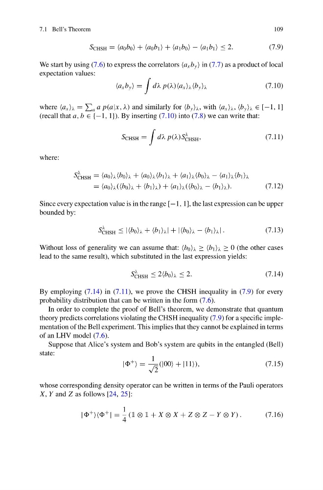
We start by using (7.6) to express the correlators a x b y in (7.7) as a product of local
expectation values:
a x b y =
dλ p(λ)a x λ b y λ
(7.10)
where a x λ =
a a p(a|x, λ) and similarly for b y λ , with a x λ , b y λ ∈ [−1, 1]
(recall that a, b ∈ {−1, 1}). By inserting (7.10) into (7.8) we can write that:
S CHSH =
dλ p(λ)S
λ
CHSH ,
(7.11)
where:
S
λ
CHSH = =a 0 λ b 0 λ + +a 0 λ b 1 λ + +a 1 λ b 0 λ − −a 1 λ b 1 λ
= =a 0 λ (b 0 λ + +b 1 λ ) + +a 1 λ (b 0 λ − −b 1 λ ).
(7.12)
Since every expectation value is in the range [−1, 1], the last expression can be upper
bounded by:
S
λ
CHSH ≤ |b 0 λ + +b 1 λ | + |b 0 λ − −b 1 λ | .
(7.13)
Without loss of generality we can assume that: b 0 λ ≥ ≥b 1 λ ≥ 0 (the other cases
lead to the same result), which substituted in the last expression yields:
S
λ
CHSH ≤ 2b 0 λ ≤ 2.
(7.14)
By employing (7.14) in (7.11), we prove the CHSH inequality in (7.9) for every
probability distribution that can be written in the form (7.6).
In order to complete the proof of Bell’s theorem, we demonstrate that quantum
theory predicts correlations violating the CHSH inequality (7.9) for a specific implementation of the Bell experiment. This implies that they cannot be explained in terms
of an LHV model (7.6).
Suppose that Alice’s system and Bob’s system are qubits in the entangled (Bell)
state:
|
+
=
1
√
2
(|00 + |11),
(7.15)
whose corresponding density operator can be written in terms of the Pauli operators
X, Y and Z as follows [24, 25]:
|
+
+
| =
1
4
(1 ⊗ 1 + X ⊗ X + Z ⊗ Z − Y ⊗ Y ) .
(7.16)
109
S CHSH = =a 0 b 0 + +a 0 b 1 + +a 1 b 0 − −a 1 b 1 ≤ 2.
(7.9)
We start by using (7.6) to express the correlators a x b y in (7.7) as a product of local
expectation values:
a x b y =
dλ p(λ)a x λ b y λ
(7.10)
where a x λ =
a a p(a|x, λ) and similarly for b y λ , with a x λ , b y λ ∈ [−1, 1]
(recall that a, b ∈ {−1, 1}). By inserting (7.10) into (7.8) we can write that:
S CHSH =
dλ p(λ)S
λ
CHSH ,
(7.11)
where:
S
λ
CHSH = =a 0 λ b 0 λ + +a 0 λ b 1 λ + +a 1 λ b 0 λ − −a 1 λ b 1 λ
= =a 0 λ (b 0 λ + +b 1 λ ) + +a 1 λ (b 0 λ − −b 1 λ ).
(7.12)
Since every expectation value is in the range [−1, 1], the last expression can be upper
bounded by:
S
λ
CHSH ≤ |b 0 λ + +b 1 λ | + |b 0 λ − −b 1 λ | .
(7.13)
Without loss of generality we can assume that: b 0 λ ≥ ≥b 1 λ ≥ 0 (the other cases
lead to the same result), which substituted in the last expression yields:
S
λ
CHSH ≤ 2b 0 λ ≤ 2.
(7.14)
By employing (7.14) in (7.11), we prove the CHSH inequality in (7.9) for every
probability distribution that can be written in the form (7.6).
In order to complete the proof of Bell’s theorem, we demonstrate that quantum
theory predicts correlations violating the CHSH inequality (7.9) for a specific implementation of the Bell experiment. This implies that they cannot be explained in terms
of an LHV model (7.6).
Suppose that Alice’s system and Bob’s system are qubits in the entangled (Bell)
state:
|
+
=
1
√
2
(|00 + |11),
(7.15)
whose corresponding density operator can be written in terms of the Pauli operators
X, Y and Z as follows [24, 25]:
|
+
+
| =
1
4
(1 ⊗ 1 + X ⊗ X + Z ⊗ Z − Y ⊗ Y ) .
(7.16)