

16 Uncertainty Treatment Applications: High-Enthalpy Flow Ground Testing
523
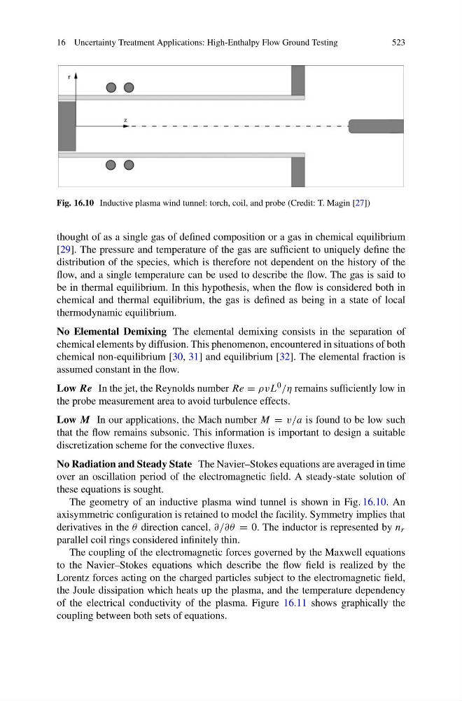
Fig. 16.10 Inductive plasma wind tunnel: torch, coil, and probe (Credit: T. Magin [27])
thought of as a single gas of defined composition or a gas in chemical equilibrium
[29]. The pressure and temperature of the gas are sufficient to uniquely define the
distribution of the species, which is therefore not dependent on the history of the
flow, and a single temperature can be used to describe the flow. The gas is said to
be in thermal equilibrium. In this hypothesis, when the flow is considered both in
chemical and thermal equilibrium, the gas is defined as being in a state of local
thermodynamic equilibrium.
No Elemental Demixing The elemental demixing consists in the separation of
chemical elements by diffusion. This phenomenon, encountered in situations of both
chemical non-equilibrium [30, 31] and equilibrium [32]. The elemental fraction is
assumed constant in the flow.
Low Re In the jet, the Reynolds number Re = ρvL 0 /η remains sufficiently low in
the probe measurement area to avoid turbulence effects.
Low M In our applications, the Mach number M = v/a is found to be low such
that the flow remains subsonic. This information is important to design a suitable
discretization scheme for the convective fluxes.
No Radiation and Steady State The Navier–Stokes equations are averaged in time
over an oscillation period of the electromagnetic field. A steady-state solution of
these equations is sought.
The geometry of an inductive plasma wind tunnel is shown in Fig. 16.10. An
axisymmetric configuration is retained to model the facility. Symmetry implies that
derivatives in the θ direction cancel, ∂/∂θ = 0. The inductor is represented by n r
parallel coil rings considered infinitely thin.
The coupling of the electromagnetic forces governed by the Maxwell equations
to the Navier–Stokes equations which describe the flow field is realized by the
Lorentz forces acting on the charged particles subject to the electromagnetic field,
the Joule dissipation which heats up the plasma, and the temperature dependency
of the electrical conductivity of the plasma. Figure 16.11 shows graphically the
coupling between both sets of equations.