

488
B. Arizmendi et al.
15.3.4.6 An Unsteady Ice Accretion Model
A model based on the exact solution of the Stefan problem accounts for the unsteady
glaze ice accretion which closely follows the Myers formulation. As previously
discussed in aeronautical working conditions the water film is very thin, thus
justifying the assumption of infinite conduction through the water. The temperature
of the liquid film can then be assumed as approximately constant and equal to the
freezing temperature of water. Dirichlet boundary conditions are then imposed on
the supposedly infinitesimally thin water layer resulting in the water layer being
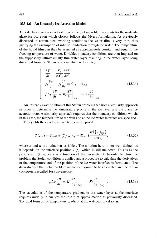
discarded from the Stefan problem which reduced to,
⎧
⎪ ⎪ ⎪ ⎪ ⎪ ⎪ ⎪ ⎪ ⎨
⎪ ⎪ ⎪ ⎪ ⎪ ⎪ ⎪ ⎪ ⎩
∂T
∂t
=
K s
ρ s C s
∂ 2 T
∂z 2
ρ s
∂B
∂t
+ ρ l
∂h
∂t
= ˙
m in − ˙
m out
ρL F
∂B
∂t
= K s
∂T
∂z
B(t) −
− K l
∂ϑ
∂z
B(t) +
.
(15.34)
An unsteady exact solution of this Stefan problem then uses a similarity approach
in order to determine the temperature profile in the ice layer and the glaze ice
accretion rate. A similarity approach requires that the boundary conditions which,
in this case, the temperature of the wall and at the ice-water interface are specified.
This yields the exact glaze ice temperature profile,
T (z, t) = T wall +
T f reezing − T wall
erf
z
2
√
α i t
erf(λ)
,
(15.35)
where λ and α are reduction variables. The solution here is not well defined as
it depends on the interface position B(t), which is still unknown. This is as the
parameter B(t) appears as a function of the parameter λ. In order to close the
problem the Stefan condition is applied and a procedure to calculate the derivatives
of the temperature and of the position of the ice-water interface is formulated. The
derivatives of the Stefan problem are hence required to be calculated and the Stefan
condition is recalled for convenience,
ρL F
∂B
∂t
= K s
∂T
∂z
B(t) −
− K l
∂ϑ
∂z
B(t) +
.
(15.36)
The calculation of the temperature gradient in the water layer at the interface
requires initially to analyze the thin film approximation as previously discussed.
The final form of the temperature gradient at the water-air interface is,
B. Arizmendi et al.
15.3.4.6 An Unsteady Ice Accretion Model
A model based on the exact solution of the Stefan problem accounts for the unsteady
glaze ice accretion which closely follows the Myers formulation. As previously
discussed in aeronautical working conditions the water film is very thin, thus
justifying the assumption of infinite conduction through the water. The temperature
of the liquid film can then be assumed as approximately constant and equal to the
freezing temperature of water. Dirichlet boundary conditions are then imposed on
the supposedly infinitesimally thin water layer resulting in the water layer being
discarded from the Stefan problem which reduced to,
⎧
⎪ ⎪ ⎪ ⎪ ⎪ ⎪ ⎪ ⎪ ⎨
⎪ ⎪ ⎪ ⎪ ⎪ ⎪ ⎪ ⎪ ⎩
∂T
∂t
=
K s
ρ s C s
∂ 2 T
∂z 2
ρ s
∂B
∂t
+ ρ l
∂h
∂t
= ˙
m in − ˙
m out
ρL F
∂B
∂t
= K s
∂T
∂z
B(t) −
− K l
∂ϑ
∂z
B(t) +
.
(15.34)
An unsteady exact solution of this Stefan problem then uses a similarity approach
in order to determine the temperature profile in the ice layer and the glaze ice
accretion rate. A similarity approach requires that the boundary conditions which,
in this case, the temperature of the wall and at the ice-water interface are specified.
This yields the exact glaze ice temperature profile,
T (z, t) = T wall +
T f reezing − T wall
erf
z
2
√
α i t
erf(λ)
,
(15.35)
where λ and α are reduction variables. The solution here is not well defined as
it depends on the interface position B(t), which is still unknown. This is as the
parameter B(t) appears as a function of the parameter λ. In order to close the
problem the Stefan condition is applied and a procedure to calculate the derivatives
of the temperature and of the position of the ice-water interface is formulated. The
derivatives of the Stefan problem are hence required to be calculated and the Stefan
condition is recalled for convenience,
ρL F
∂B
∂t
= K s
∂T
∂z
B(t) −
− K l
∂ϑ
∂z
B(t) +
.
(15.36)
The calculation of the temperature gradient in the water layer at the interface
requires initially to analyze the thin film approximation as previously discussed.
The final form of the temperature gradient at the water-air interface is,