

15 In-flight Icing: Modeling, Prediction, and Uncertainty
477
accretion rates. Physical phenomenon such as the transition of the boundary layer
as well as its detachment have an effect of the convective heat transfer fluxes. The
study of these factors should be carefully considered [6]. However, determining the
most accurate method for modeling the aerodynamic flow field in icing conditions is
under discussion. Ideally, the prerequisite for the solver should be that it is capable
of handling complex aircraft and ice geometries and complicated flows. Severe
ice accretion scenarios that present complex and large ice formations poses a big
challenge for the develompent of computational models. An example are the ice
horns such as the ones described in Sect. 15.2.3, pose large challenges for many
computational methods. The abnormally large and inherently irregular increase in
roughness also something that methods should be able to account for.
15.3.1.1 Flow Solver
Commonplace aerodynamic flow field prediction methods implement various ways
of modeling. Examples of these techniques are linear panel methods with integral
boundaries [70], interactive boundary layer representation [71] and ReynoldsAveraged Navier-Stokes simulations (RANS) [72]. These metods present different
levels of complexity and accuracy. Precise predictions of flow features for a range
of geometries and flow conditions are a mandatory goal for flow solvers. For
icing purposes, the flow solver is required to reliably predict separation onsets
and progressions in highly curved surfaces [6]. With complex ice structures,
such as horns, this becomes very challenging. RANS simulations are the most
widespread modeling approach for fast and generally reliable predictions of flow
field. Reynolds-Averaged Navier-Stokes (RANS) equations require a turbulence
model. This decomposition of the Navier-Stokes equations into the RANS equations
introduces a set of unknowns called Reynolds Stresses, which are functions of
the velocity fluctuations and utilize a turbulence model for closure of the system
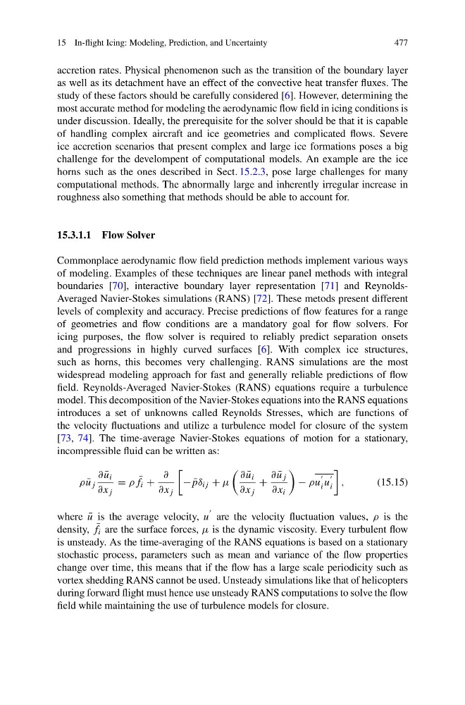
[73, 74]. The time-average Navier-Stokes equations of motion for a stationary,
incompressible fluid can be written as:
ρ ¯
u j
∂ ¯
u i
∂x j
= ρ ¯
f i +
∂
∂x j
− ¯
pδ ij + μ
∂ ¯
u i
∂x j
+
∂ ¯
u j
∂x i
− ρu
i u
i
,
(15.15)
where ¯
u is the average velocity, u
are the velocity fluctuation values, ρ is the
density, ¯
f i are the surface forces, μ is the dynamic viscosity. Every turbulent flow
is unsteady. As the time-averaging of the RANS equations is based on a stationary
stochastic process, parameters such as mean and variance of the flow properties
change over time, this means that if the flow has a large scale periodicity such as
vortex shedding RANS cannot be used. Unsteady simulations like that of helicopters
during forward flight must hence use unsteady RANS computations to solve the flow
field while maintaining the use of turbulence models for closure.
477
accretion rates. Physical phenomenon such as the transition of the boundary layer
as well as its detachment have an effect of the convective heat transfer fluxes. The
study of these factors should be carefully considered [6]. However, determining the
most accurate method for modeling the aerodynamic flow field in icing conditions is
under discussion. Ideally, the prerequisite for the solver should be that it is capable
of handling complex aircraft and ice geometries and complicated flows. Severe
ice accretion scenarios that present complex and large ice formations poses a big
challenge for the develompent of computational models. An example are the ice
horns such as the ones described in Sect. 15.2.3, pose large challenges for many
computational methods. The abnormally large and inherently irregular increase in
roughness also something that methods should be able to account for.
15.3.1.1 Flow Solver
Commonplace aerodynamic flow field prediction methods implement various ways
of modeling. Examples of these techniques are linear panel methods with integral
boundaries [70], interactive boundary layer representation [71] and ReynoldsAveraged Navier-Stokes simulations (RANS) [72]. These metods present different
levels of complexity and accuracy. Precise predictions of flow features for a range
of geometries and flow conditions are a mandatory goal for flow solvers. For
icing purposes, the flow solver is required to reliably predict separation onsets
and progressions in highly curved surfaces [6]. With complex ice structures,
such as horns, this becomes very challenging. RANS simulations are the most
widespread modeling approach for fast and generally reliable predictions of flow
field. Reynolds-Averaged Navier-Stokes (RANS) equations require a turbulence
model. This decomposition of the Navier-Stokes equations into the RANS equations
introduces a set of unknowns called Reynolds Stresses, which are functions of
the velocity fluctuations and utilize a turbulence model for closure of the system
[73, 74]. The time-average Navier-Stokes equations of motion for a stationary,
incompressible fluid can be written as:
ρ ¯
u j
∂ ¯
u i
∂x j
= ρ ¯
f i +
∂
∂x j
− ¯
pδ ij + μ
∂ ¯
u i
∂x j
+
∂ ¯
u j
∂x i
− ρu
i u
i
,
(15.15)
where ¯
u is the average velocity, u
are the velocity fluctuation values, ρ is the
density, ¯
f i are the surface forces, μ is the dynamic viscosity. Every turbulent flow
is unsteady. As the time-averaging of the RANS equations is based on a stationary
stochastic process, parameters such as mean and variance of the flow properties
change over time, this means that if the flow has a large scale periodicity such as
vortex shedding RANS cannot be used. Unsteady simulations like that of helicopters
during forward flight must hence use unsteady RANS computations to solve the flow
field while maintaining the use of turbulence models for closure.