

13 Risk Measures in the Context of Robust and Reliability Based Optimization
419
13.4.1 Estimation of Risk Functions Using ECDF
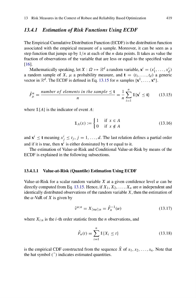
The Empirical Cumulative Distribution Function (ECDF) is the distribution function
associated with the empirical measure of a sample. Moreover, it can be seen as a
step function that jumps up by 1/n at each of the n data points. It takes as value the
fraction of observations of the variable that are less or equal to the specified value
[16].
Mathematically speaking, let X : Ω → R d a random variable, x i = (x i
1 , . . . , x i
d )
a random sample of X, μ a probability measure, and t = (t 1 , . . . , t d ) a generic
vector in R d . The ECDF is defined in Eq. 13.15 for n samples {x 1 , . . . , x n }.
ˆ
F
n
μ =
number of elements in the sample ≤ t
n
=
1
n
n
i=1
1{x
i
≤ t}
(13.15)
where 1{A} is the indicator of event A:
1 A (x) :=
1 if x ∈ A
0 if x /
∈ A
(13.16)
and x i ≤ t meaning x i
j ≤ t j , j = 1, . . . , d. The last relation defines a partial order
and if it is true, then x i is either dominated by t or equal to it.
The estimation of Value-at-Risk and Conditional Value-at-Risk by means of the
ECDF is explained in the following subsections.
13.4.1.1 Value-at-Risk (Quantile) Estimation Using ECDF
Value-at-Risk for a scalar random variable X at a given confidence level α can be
directly computed from Eq. 13.15. Hence, if X 1 , X 2 , . . . , X n are n independent and
identically distributed observations of the random variable X, then the estimation of
the α-VaR of X is given by
ˆ
ν
α;n
= X nα:n = ˆ
F
−1
n (α)
(13.17)
where X i:n is the i-th order statistic from the n observations, and
ˆ
F n (t) =
n
i=1
1{X i ≤ t}
(13.18)
is the empirical CDF constructed from the sequence ˜
X of x 1 , x 2 , . . . , x n . Note that
the hat symbol ( ˆ ) indicates estimated quantities.
419
13.4.1 Estimation of Risk Functions Using ECDF
The Empirical Cumulative Distribution Function (ECDF) is the distribution function
associated with the empirical measure of a sample. Moreover, it can be seen as a
step function that jumps up by 1/n at each of the n data points. It takes as value the
fraction of observations of the variable that are less or equal to the specified value
[16].
Mathematically speaking, let X : Ω → R d a random variable, x i = (x i
1 , . . . , x i
d )
a random sample of X, μ a probability measure, and t = (t 1 , . . . , t d ) a generic
vector in R d . The ECDF is defined in Eq. 13.15 for n samples {x 1 , . . . , x n }.
ˆ
F
n
μ =
number of elements in the sample ≤ t
n
=
1
n
n
i=1
1{x
i
≤ t}
(13.15)
where 1{A} is the indicator of event A:
1 A (x) :=
1 if x ∈ A
0 if x /
∈ A
(13.16)
and x i ≤ t meaning x i
j ≤ t j , j = 1, . . . , d. The last relation defines a partial order
and if it is true, then x i is either dominated by t or equal to it.
The estimation of Value-at-Risk and Conditional Value-at-Risk by means of the
ECDF is explained in the following subsections.
13.4.1.1 Value-at-Risk (Quantile) Estimation Using ECDF
Value-at-Risk for a scalar random variable X at a given confidence level α can be
directly computed from Eq. 13.15. Hence, if X 1 , X 2 , . . . , X n are n independent and
identically distributed observations of the random variable X, then the estimation of
the α-VaR of X is given by
ˆ
ν
α;n
= X nα:n = ˆ
F
−1
n (α)
(13.17)
where X i:n is the i-th order statistic from the n observations, and
ˆ
F n (t) =
n
i=1
1{X i ≤ t}
(13.18)
is the empirical CDF constructed from the sequence ˜
X of x 1 , x 2 , . . . , x n . Note that
the hat symbol ( ˆ ) indicates estimated quantities.