

416
E. M. Tirado and D. Quagliarella
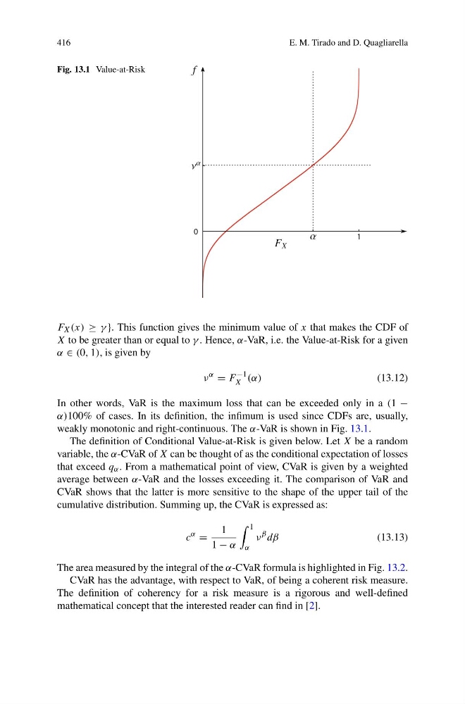
Fig. 13.1 Value-at-Risk
1
0
F X (x) ≥ γ }. This function gives the minimum value of x that makes the CDF of
X to be greater than or equal to γ . Hence, α-VaR, i.e. the Value-at-Risk for a given
α ∈ (0, 1), is given by
ν
α
= F
−1
X (α)
(13.12)
In other words, VaR is the maximum loss that can be exceeded only in a (1 −
α)100% of cases. In its definition, the infimum is used since CDFs are, usually,
weakly monotonic and right-continuous. The α-VaR is shown in Fig. 13.1.
The definition of Conditional Value-at-Risk is given below. Let X be a random
variable, the α-CVaR of X can be thought of as the conditional expectation of losses
that exceed q α . From a mathematical point of view, CVaR is given by a weighted
average between α-VaR and the losses exceeding it. The comparison of VaR and
CVaR shows that the latter is more sensitive to the shape of the upper tail of the
cumulative distribution. Summing up, the CVaR is expressed as:
c
α
=
1
1 − α
1
α
ν
β dβ
(13.13)
The area measured by the integral of the α-CVaR formula is highlighted in Fig. 13.2.
CVaR has the advantage, with respect to VaR, of being a coherent risk measure.
The definition of coherency for a risk measure is a rigorous and well-defined
mathematical concept that the interested reader can find in [2].
E. M. Tirado and D. Quagliarella
Fig. 13.1 Value-at-Risk
1
0
F X (x) ≥ γ }. This function gives the minimum value of x that makes the CDF of
X to be greater than or equal to γ . Hence, α-VaR, i.e. the Value-at-Risk for a given
α ∈ (0, 1), is given by
ν
α
= F
−1
X (α)
(13.12)
In other words, VaR is the maximum loss that can be exceeded only in a (1 −
α)100% of cases. In its definition, the infimum is used since CDFs are, usually,
weakly monotonic and right-continuous. The α-VaR is shown in Fig. 13.1.
The definition of Conditional Value-at-Risk is given below. Let X be a random
variable, the α-CVaR of X can be thought of as the conditional expectation of losses
that exceed q α . From a mathematical point of view, CVaR is given by a weighted
average between α-VaR and the losses exceeding it. The comparison of VaR and
CVaR shows that the latter is more sensitive to the shape of the upper tail of the
cumulative distribution. Summing up, the CVaR is expressed as:
c
α
=
1
1 − α
1
α
ν
β dβ
(13.13)
The area measured by the integral of the α-CVaR formula is highlighted in Fig. 13.2.
CVaR has the advantage, with respect to VaR, of being a coherent risk measure.
The definition of coherency for a risk measure is a rigorous and well-defined
mathematical concept that the interested reader can find in [2].