

12 Response Surface Methodology
407
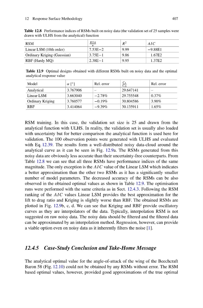
Table 12.8 Performance indices of RSMs built on noisy data (the validation set of 25 samples were
drawn with ULHS from the analytical) function
RSM
RSA
n
R 2
AI C
Linear LSM (10th order)
7.53E−2
9.99
−9.88E1
Ordinary Kriging (Gaussian)
3.75E−1
9.86
1.67E2
RBF (Hardy MQ)
2.38E−1
9.95
1.37E2
Table 12.9 Optimal designs obtained with different RSMs built on noisy data and the optimal
analytical response value
Model
α [ ◦ ]
Rel. error
C L
C D
Rel. error
Analytical
3.767906
–
29.647141
–
Linear LSM
3.663040
−2.78%
29.755548
0.37%
Ordinary Kriging
3.760577
−0.19%
30.804586
3.90%
RBF
3.414064
−9.39%
30.135911
1.65%
RSM training. In this case, the validation set size is 25 and drawn from the
analytical function with ULHS. In reality, the validation set is usually also loaded
with uncertainty but for better comparison the analytical function is used here for
validation. The 100 observation points were generated with ULHS and evaluated
with Eq. 12.39. The results form a well-distributed noisy data-cloud around the
analytical curve as it can be seen in Fig. 12.9a. The RSMs generated from this
noisy data are obviously less accurate than their uncertainty-free counterparts. From
Table 12.8 we can see that all three RSMs have performance indices of the same
magnitude. The only exception is the AI C value of the Linear LSM which indicates
a better approximation than the other two RSMs as it has a significantly smaller
number of model parameters. The decreased accuracy of the RSMs can be also
observed in the obtained optimal values as shown in Table 12.9. The optimisation
runs were performed with the same criteria as in Sect. 12.4.3. Following the RSM
ranking of the AI C values Linear LSM provides the best approximation for the
lift to drag ratio and Kriging is slightly worse than RBF. The obtained RSMs are
plotted in Fig. 12.9b, c, d. We can see that Kriging and RBF provide oscillatory
curves as they are interpolators of the data. Typically, interpolation RSM is not
suggested on raw noisy data. The noisy data should be filtered and the filtered data
can be approximated by an interpolation method. Regression, however, can provide
a viable option even on noisy data as it inherently filters the noise [1].
12.4.5 Case-Study Conclusion and Take-Home Message
The analytical optimal value for the angle-of-attack of the wing of the Beechcraft
Baron 58 (Fig. 12.10) could not be obtained by any RSMs without error. The RSM
based optimal values, however, provided good approximations of the true optimal
407
Table 12.8 Performance indices of RSMs built on noisy data (the validation set of 25 samples were
drawn with ULHS from the analytical) function
RSM
RSA
n
R 2
AI C
Linear LSM (10th order)
7.53E−2
9.99
−9.88E1
Ordinary Kriging (Gaussian)
3.75E−1
9.86
1.67E2
RBF (Hardy MQ)
2.38E−1
9.95
1.37E2
Table 12.9 Optimal designs obtained with different RSMs built on noisy data and the optimal
analytical response value
Model
α [ ◦ ]
Rel. error
C L
C D
Rel. error
Analytical
3.767906
–
29.647141
–
Linear LSM
3.663040
−2.78%
29.755548
0.37%
Ordinary Kriging
3.760577
−0.19%
30.804586
3.90%
RBF
3.414064
−9.39%
30.135911
1.65%
RSM training. In this case, the validation set size is 25 and drawn from the
analytical function with ULHS. In reality, the validation set is usually also loaded
with uncertainty but for better comparison the analytical function is used here for
validation. The 100 observation points were generated with ULHS and evaluated
with Eq. 12.39. The results form a well-distributed noisy data-cloud around the
analytical curve as it can be seen in Fig. 12.9a. The RSMs generated from this
noisy data are obviously less accurate than their uncertainty-free counterparts. From
Table 12.8 we can see that all three RSMs have performance indices of the same
magnitude. The only exception is the AI C value of the Linear LSM which indicates
a better approximation than the other two RSMs as it has a significantly smaller
number of model parameters. The decreased accuracy of the RSMs can be also
observed in the obtained optimal values as shown in Table 12.9. The optimisation
runs were performed with the same criteria as in Sect. 12.4.3. Following the RSM
ranking of the AI C values Linear LSM provides the best approximation for the
lift to drag ratio and Kriging is slightly worse than RBF. The obtained RSMs are
plotted in Fig. 12.9b, c, d. We can see that Kriging and RBF provide oscillatory
curves as they are interpolators of the data. Typically, interpolation RSM is not
suggested on raw noisy data. The noisy data should be filtered and the filtered data
can be approximated by an interpolation method. Regression, however, can provide
a viable option even on noisy data as it inherently filters the noise [1].
12.4.5 Case-Study Conclusion and Take-Home Message
The analytical optimal value for the angle-of-attack of the wing of the Beechcraft
Baron 58 (Fig. 12.10) could not be obtained by any RSMs without error. The RSM
based optimal values, however, provided good approximations of the true optimal