

12 Response Surface Methodology
405
Table 12.7 Performance indices of different RBF models of the lift to drag ratio. The validation
set consists of 10 samples generated with ULHS
RSM
RSA
n
R 2
AI C
RBF-25 (random)
3.55E−7
1.000
−2.34E2
RBF-50 (random)
5.47E−8
1.000
−2.16E2
RBF-100 (random)
9.05E−9
1.000
−1.63E2
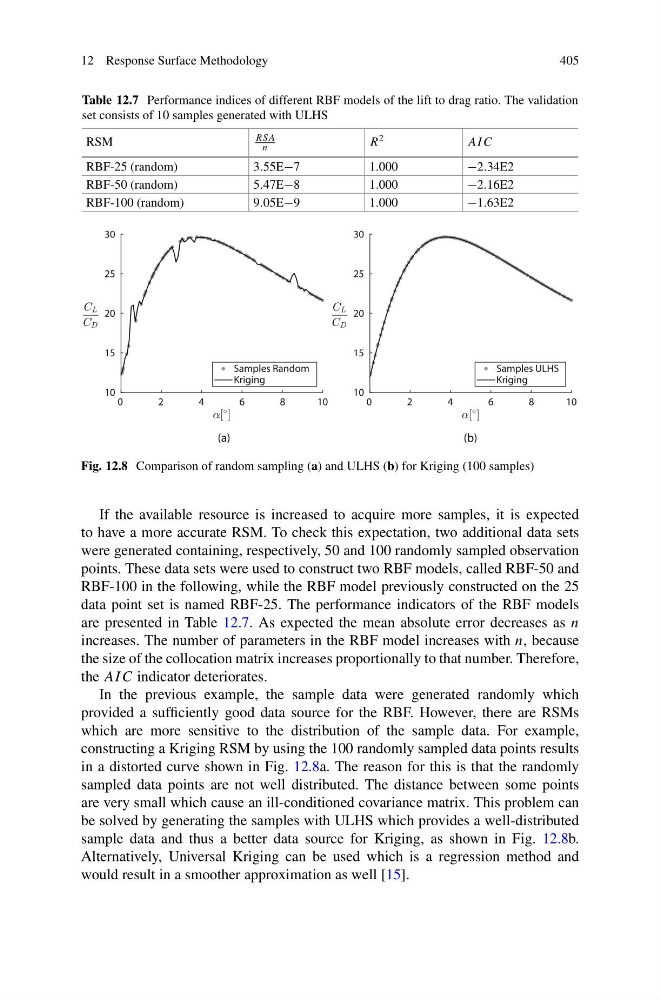
Fig. 12.8 Comparison of random sampling (a) and ULHS (b) for Kriging (100 samples)
If the available resource is increased to acquire more samples, it is expected
to have a more accurate RSM. To check this expectation, two additional data sets
were generated containing, respectively, 50 and 100 randomly sampled observation
points. These data sets were used to construct two RBF models, called RBF-50 and
RBF-100 in the following, while the RBF model previously constructed on the 25
data point set is named RBF-25. The performance indicators of the RBF models
are presented in Table 12.7. As expected the mean absolute error decreases as n
increases. The number of parameters in the RBF model increases with n, because
the size of the collocation matrix increases proportionally to that number. Therefore,
the AI C indicator deteriorates.
In the previous example, the sample data were generated randomly which
provided a sufficiently good data source for the RBF. However, there are RSMs
which are more sensitive to the distribution of the sample data. For example,
constructing a Kriging RSM by using the 100 randomly sampled data points results
in a distorted curve shown in Fig. 12.8a. The reason for this is that the randomly
sampled data points are not well distributed. The distance between some points
are very small which cause an ill-conditioned covariance matrix. This problem can
be solved by generating the samples with ULHS which provides a well-distributed
sample data and thus a better data source for Kriging, as shown in Fig. 12.8b.
Alternatively, Universal Kriging can be used which is a regression method and
would result in a smoother approximation as well [15].
405
Table 12.7 Performance indices of different RBF models of the lift to drag ratio. The validation
set consists of 10 samples generated with ULHS
RSM
RSA
n
R 2
AI C
RBF-25 (random)
3.55E−7
1.000
−2.34E2
RBF-50 (random)
5.47E−8
1.000
−2.16E2
RBF-100 (random)
9.05E−9
1.000
−1.63E2
Fig. 12.8 Comparison of random sampling (a) and ULHS (b) for Kriging (100 samples)
If the available resource is increased to acquire more samples, it is expected
to have a more accurate RSM. To check this expectation, two additional data sets
were generated containing, respectively, 50 and 100 randomly sampled observation
points. These data sets were used to construct two RBF models, called RBF-50 and
RBF-100 in the following, while the RBF model previously constructed on the 25
data point set is named RBF-25. The performance indicators of the RBF models
are presented in Table 12.7. As expected the mean absolute error decreases as n
increases. The number of parameters in the RBF model increases with n, because
the size of the collocation matrix increases proportionally to that number. Therefore,
the AI C indicator deteriorates.
In the previous example, the sample data were generated randomly which
provided a sufficiently good data source for the RBF. However, there are RSMs
which are more sensitive to the distribution of the sample data. For example,
constructing a Kriging RSM by using the 100 randomly sampled data points results
in a distorted curve shown in Fig. 12.8a. The reason for this is that the randomly
sampled data points are not well distributed. The distance between some points
are very small which cause an ill-conditioned covariance matrix. This problem can
be solved by generating the samples with ULHS which provides a well-distributed
sample data and thus a better data source for Kriging, as shown in Fig. 12.8b.
Alternatively, Universal Kriging can be used which is a regression method and
would result in a smoother approximation as well [15].