

12 Response Surface Methodology
397
see the work of Rasmussen and Williams [8]. Forrester et al. book [1] discusses
the methodology from an engineering point of view, whereas Cressie [9] puts the
discussion into the original geostatistical context.
A GP regression model approximates the response as a stochastic process,
ˆ
f (x) ∼ GP (μ(x), k(x, x
)),
(12.21)
where GP (.) means a Gaussian Process function, i.e. any finite linear combination
of random variables with Gaussian joint probability density function. μ(x) denotes
the trend or the mean and represents the global variations of the response, while
k(x, x ) is the covariance function and represents the local variations of the response.
In principle, any GP can be completely described by its second-order statistics,
i.e. the mean and covariance functions. In addition to the global trend and local
departure, the model can be extended by a white noise term in the event of noisy
observations, in which case, the RSM can be formulated as follows:
ˆ
f (x) = μ(x) + δ(x) + (x),
(12.22)
where μ(x) is the global trend, δ(x) is the local departure, and (x) is the white
noise function, respectively. Both local departure and white noise terms have zero
mean and constant variance.
In Ordinary Kriging, the mean function is constant and the local departure is
stationary and depends only on the spatial difference of the samples. In practice, the
white noise term is incorporated into the local departure term through an offset of
the variogram, which is discussed in Sect. 12.3.3.1. Ordinary Kriging interpolates
the response values as a linear combination of the observed values,
ˆ
f (x) = λ
T f,
(12.23)
where λ are the weight parameters so that
λ i = 1. The weights contain the term
of local departure and as a result depend on the spatial difference of the training
points and the predicted points. The optimal weights are computed by looking for
the Best Linear Unbiased Estimator by minimising the Mean Squared Error of the
predictor,
min
λ
E[| ˆ
f (x ∗ ) − f (x ∗ )|
2
],
(12.24)
where x ∗ is the location of the predicted value. The unbiasedness means that the
approximation model and the true function evaluations have the same expected
value (see Ref. [10]).
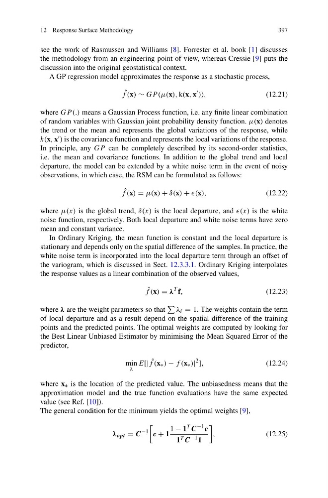
The general condition for the minimum yields the optimal weights [9],
λ opt = C
−1
c + 1
1 − 1 T C
−1 c
1 T C
−1 1
,
(12.25)
397
see the work of Rasmussen and Williams [8]. Forrester et al. book [1] discusses
the methodology from an engineering point of view, whereas Cressie [9] puts the
discussion into the original geostatistical context.
A GP regression model approximates the response as a stochastic process,
ˆ
f (x) ∼ GP (μ(x), k(x, x
)),
(12.21)
where GP (.) means a Gaussian Process function, i.e. any finite linear combination
of random variables with Gaussian joint probability density function. μ(x) denotes
the trend or the mean and represents the global variations of the response, while
k(x, x ) is the covariance function and represents the local variations of the response.
In principle, any GP can be completely described by its second-order statistics,
i.e. the mean and covariance functions. In addition to the global trend and local
departure, the model can be extended by a white noise term in the event of noisy
observations, in which case, the RSM can be formulated as follows:
ˆ
f (x) = μ(x) + δ(x) + (x),
(12.22)
where μ(x) is the global trend, δ(x) is the local departure, and (x) is the white
noise function, respectively. Both local departure and white noise terms have zero
mean and constant variance.
In Ordinary Kriging, the mean function is constant and the local departure is
stationary and depends only on the spatial difference of the samples. In practice, the
white noise term is incorporated into the local departure term through an offset of
the variogram, which is discussed in Sect. 12.3.3.1. Ordinary Kriging interpolates
the response values as a linear combination of the observed values,
ˆ
f (x) = λ
T f,
(12.23)
where λ are the weight parameters so that
λ i = 1. The weights contain the term
of local departure and as a result depend on the spatial difference of the training
points and the predicted points. The optimal weights are computed by looking for
the Best Linear Unbiased Estimator by minimising the Mean Squared Error of the
predictor,
min
λ
E[| ˆ
f (x ∗ ) − f (x ∗ )|
2
],
(12.24)
where x ∗ is the location of the predicted value. The unbiasedness means that the
approximation model and the true function evaluations have the same expected
value (see Ref. [10]).
The general condition for the minimum yields the optimal weights [9],
λ opt = C
−1
c + 1
1 − 1 T C
−1 c
1 T C
−1 1
,
(12.25)