

12 Response Surface Methodology
395
α = (X
T X)
−1 X
T y.
(12.15)
In the case of a Nonlinear Least Squares Problem the Eq. (12.11) is approximated
and the coefficients are traditionally found by an iterative method such as the Gauss–
Newton, Levenberg–Marquardt or Genetic Algorithms.
12.3.2 Radial Basis Functions
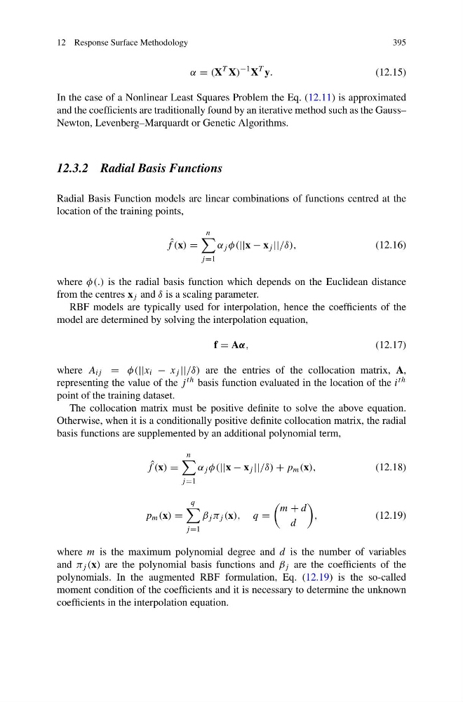
Radial Basis Function models are linear combinations of functions centred at the
location of the training points,
ˆ
f (x) =
n
j =1
α j φ(||x − x j ||/δ),
(12.16)
where φ(.) is the radial basis function which depends on the Euclidean distance
from the centres x j and δ is a scaling parameter.
RBF models are typically used for interpolation, hence the coefficients of the
model are determined by solving the interpolation equation,
f = Aα,
(12.17)
where A ij = φ(||x i − x j ||/δ) are the entries of the collocation matrix, A,
representing the value of the j th basis function evaluated in the location of the i th
point of the training dataset.
The collocation matrix must be positive definite to solve the above equation.
Otherwise, when it is a conditionally positive definite collocation matrix, the radial
basis functions are supplemented by an additional polynomial term,
ˆ
f (x) =
n
j =1
α j φ(||x − x j ||/δ) + p m (x),
(12.18)
p m (x) =
q
j =1
β j π j (x), q =
m + d
d
,
(12.19)
where m is the maximum polynomial degree and d is the number of variables
and π j (x) are the polynomial basis functions and β j are the coefficients of the
polynomials. In the augmented RBF formulation, Eq. (12.19) is the so-called
moment condition of the coefficients and it is necessary to determine the unknown
coefficients in the interpolation equation.
395
α = (X
T X)
−1 X
T y.
(12.15)
In the case of a Nonlinear Least Squares Problem the Eq. (12.11) is approximated
and the coefficients are traditionally found by an iterative method such as the Gauss–
Newton, Levenberg–Marquardt or Genetic Algorithms.
12.3.2 Radial Basis Functions
Radial Basis Function models are linear combinations of functions centred at the
location of the training points,
ˆ
f (x) =
n
j =1
α j φ(||x − x j ||/δ),
(12.16)
where φ(.) is the radial basis function which depends on the Euclidean distance
from the centres x j and δ is a scaling parameter.
RBF models are typically used for interpolation, hence the coefficients of the
model are determined by solving the interpolation equation,
f = Aα,
(12.17)
where A ij = φ(||x i − x j ||/δ) are the entries of the collocation matrix, A,
representing the value of the j th basis function evaluated in the location of the i th
point of the training dataset.
The collocation matrix must be positive definite to solve the above equation.
Otherwise, when it is a conditionally positive definite collocation matrix, the radial
basis functions are supplemented by an additional polynomial term,
ˆ
f (x) =
n
j =1
α j φ(||x − x j ||/δ) + p m (x),
(12.18)
p m (x) =
q
j =1
β j π j (x), q =
m + d
d
,
(12.19)
where m is the maximum polynomial degree and d is the number of variables
and π j (x) are the polynomial basis functions and β j are the coefficients of the
polynomials. In the augmented RBF formulation, Eq. (12.19) is the so-called
moment condition of the coefficients and it is necessary to determine the unknown
coefficients in the interpolation equation.