

12 Response Surface Methodology
393
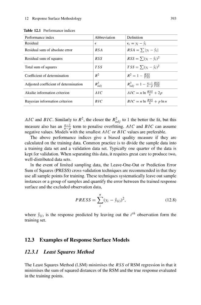
Table 12.1 Performance indices
Performance index
Abbreviation
Definition
Residual
i = y i − ˆ
y i
Residual sum of absolute error
RSA
RSA =
|y i − ˆ
y i |
Residual sum of squares
RSS
RSS =
(y i − ˆ
y i ) 2
Total sum of squares
T SS
T SS =
(y i − ¯
y i ) 2
Coefficient of determination
R 2
R 2 = 1 −
RSS
T SS
Adjusted coefficient of determination
R 2
adj
R 2
adj = 1 −
n−1
n−p
RSS
T SS
Akaike information criterion
AI C
AI C = n ln
RSS
n + 2p
Bayesian information criterion
BI C
BI C = n ln
RSS
n + p ln n
AI C and BI C. Similarly to R 2 , the closer the R 2
adj to 1 the better the fit, but this
measure also has an
n−1
n−p term to penalise overfitting. AI C and BI C can assume
negative values. Models with the smallest AI C or BI C values are preferable.
The above performance indices give a biased quality measure if they are
calculated on the training data. Common practice is to divide the sample data into
a training data set and a validation data set. Typically one quarter of the data is
kept for validation. When separating this data, it requires great care to produce two,
well-distributed data sets.
In the event of limited sampling data, the Leave-One-Out or Prediction Error
Sum of Squares (PRESS) cross-validation techniques are recommended in that they
use all sample points for training. These techniques systematically leave out sample
instances or a group of samples and quantify the error between the trained response
surface and the excluded observation data,
P RESS =
n
i
(y i − ˆ
y (i) )
2 ,
(12.8)
where ˆ
y (i) is the response predicted by leaving out the i th observation form the
training set.
12.3 Examples of Response Surface Models
12.3.1 Least Squares Method
The Least Squares Method (LSM) minimises the RSS of RSM regression in that it
minimises the sum of squared distances of the RSM and the true response evaluated
in the training points.
393
Table 12.1 Performance indices
Performance index
Abbreviation
Definition
Residual
i = y i − ˆ
y i
Residual sum of absolute error
RSA
RSA =
|y i − ˆ
y i |
Residual sum of squares
RSS
RSS =
(y i − ˆ
y i ) 2
Total sum of squares
T SS
T SS =
(y i − ¯
y i ) 2
Coefficient of determination
R 2
R 2 = 1 −
RSS
T SS
Adjusted coefficient of determination
R 2
adj
R 2
adj = 1 −
n−1
n−p
RSS
T SS
Akaike information criterion
AI C
AI C = n ln
RSS
n + 2p
Bayesian information criterion
BI C
BI C = n ln
RSS
n + p ln n
AI C and BI C. Similarly to R 2 , the closer the R 2
adj to 1 the better the fit, but this
measure also has an
n−1
n−p term to penalise overfitting. AI C and BI C can assume
negative values. Models with the smallest AI C or BI C values are preferable.
The above performance indices give a biased quality measure if they are
calculated on the training data. Common practice is to divide the sample data into
a training data set and a validation data set. Typically one quarter of the data is
kept for validation. When separating this data, it requires great care to produce two,
well-distributed data sets.
In the event of limited sampling data, the Leave-One-Out or Prediction Error
Sum of Squares (PRESS) cross-validation techniques are recommended in that they
use all sample points for training. These techniques systematically leave out sample
instances or a group of samples and quantify the error between the trained response
surface and the excluded observation data,
P RESS =
n
i
(y i − ˆ
y (i) )
2 ,
(12.8)
where ˆ
y (i) is the response predicted by leaving out the i th observation form the
training set.
12.3 Examples of Response Surface Models
12.3.1 Least Squares Method
The Least Squares Method (LSM) minimises the RSS of RSM regression in that it
minimises the sum of squared distances of the RSM and the true response evaluated
in the training points.