

11 Parameter Control in Evolutionary Optimisation
369
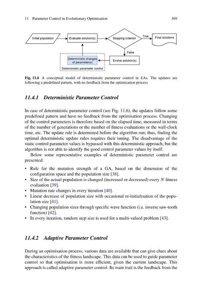
Fig. 11.6 A conceptual model of deterministic parameter control in EAs. The updates are
following a predefined pattern, with no feedback from the optimisation process
11.4.1 Deterministic Parameter Control
In case of deterministic parameter control (see Fig. 11.6), the updates follow some
predefined pattern and have no feedback from the optimisation process. Changing
of the control parameters is therefore based on the elapsed time, measured in terms
of the number of generations or the number of fitness evaluations or the wall-clock
time, etc. The update rule is determined before the algorithm run; thus, finding the
optimal deterministic update rules requires their tuning. The disadvantage of the
static control parameter values is bypassed with this deterministic approach, but the
algorithm is not able to identify the good control parameter values by itself.
Below some representative examples of deterministic parameter control are
presented:
• Rule for the mutation strength of a GA, based on the dimension of the
configuration space and the population size [38].
• Size of the actual population is changed (increased or decreased) every N fitness
evaluation [39].
• Mutation rate changes in every iteration [40].
• Linear decrease of population size with occasional re-initialisation of the population size [41].
• Changing population sizes through specific wave function (i.e. inverse saw-tooth
function) [42].
• In every iteration, random step size is used for a multi-valued problem [43].
11.4.2 Adaptive Parameter Control
During an optimisation process, various data are available that can give clues about
the characteristics of the fitness landscape. This data can be used to guide parameter
control so that optimisation is more efficient, given the current landscape. This
approach is called adaptive parameter control. Its main trait is the feedback from the
369
Fig. 11.6 A conceptual model of deterministic parameter control in EAs. The updates are
following a predefined pattern, with no feedback from the optimisation process
11.4.1 Deterministic Parameter Control
In case of deterministic parameter control (see Fig. 11.6), the updates follow some
predefined pattern and have no feedback from the optimisation process. Changing
of the control parameters is therefore based on the elapsed time, measured in terms
of the number of generations or the number of fitness evaluations or the wall-clock
time, etc. The update rule is determined before the algorithm run; thus, finding the
optimal deterministic update rules requires their tuning. The disadvantage of the
static control parameter values is bypassed with this deterministic approach, but the
algorithm is not able to identify the good control parameter values by itself.
Below some representative examples of deterministic parameter control are
presented:
• Rule for the mutation strength of a GA, based on the dimension of the
configuration space and the population size [38].
• Size of the actual population is changed (increased or decreased) every N fitness
evaluation [39].
• Mutation rate changes in every iteration [40].
• Linear decrease of population size with occasional re-initialisation of the population size [41].
• Changing population sizes through specific wave function (i.e. inverse saw-tooth
function) [42].
• In every iteration, random step size is used for a multi-valued problem [43].
11.4.2 Adaptive Parameter Control
During an optimisation process, various data are available that can give clues about
the characteristics of the fitness landscape. This data can be used to guide parameter
control so that optimisation is more efficient, given the current landscape. This
approach is called adaptive parameter control. Its main trait is the feedback from the