

352
L. Gentile et al.
b)
d)
80
0
2
4
6
8
10
y
1500
1500
1000
500
500
t(z)
t(z)
60
40
20
0
-20
-40
-60
-80
500
1000
2000
1500
t(z)
t(z)
t(z)
10
8
6
4
2
0
-50
0
50
2500
2000
t(z)1500
500
-50
0
50
80
60
40
20
0
-20
-40
-60
-80
2000
1500
500
10
8
6
4
2
Y
X
X
X
Y
Y
X
0
0
2
4
6
8
10
c)
a)
1000
3000
1000
1000
2500
2500
500
1000
1500
2000
2500
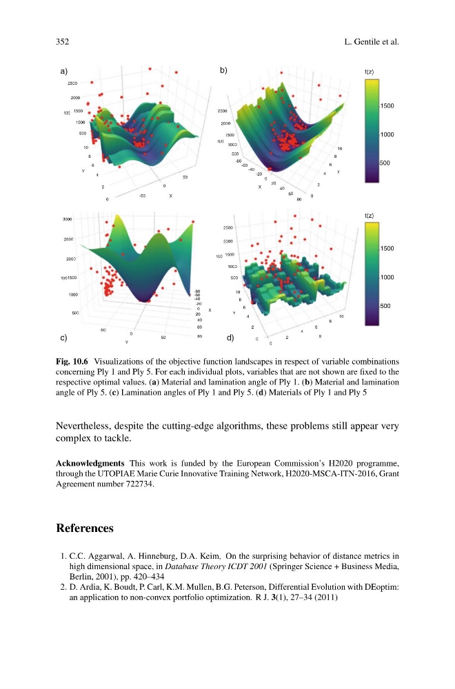
Fig. 10.6 Visualizations of the objective function landscapes in respect of variable combinations
concerning Ply 1 and Ply 5. For each individual plots, variables that are not shown are fixed to the
respective optimal values. (a) Material and lamination angle of Ply 1. (b) Material and lamination
angle of Ply 5. (c) Lamination angles of Ply 1 and Ply 5. (d) Materials of Ply 1 and Ply 5
Nevertheless, despite the cutting-edge algorithms, these problems still appear very
complex to tackle.
Acknowledgments This work is funded by the European Commission’s H2020 programme,
through the UTOPIAE Marie Curie Innovative Training Network, H2020-MSCA-ITN-2016, Grant
Agreement number 722734.
References
1. C.C. Aggarwal, A. Hinneburg, D.A. Keim, On the surprising behavior of distance metrics in
high dimensional space, in Database Theory ICDT 2001 (Springer Science + Business Media,
Berlin, 2001), pp. 420–434
2. D. Ardia, K. Boudt, P. Carl, K.M. Mullen, B.G. Peterson, Differential Evolution with DEoptim:
an application to non-convex portfolio optimization. R J. 3(1), 27–34 (2011)
L. Gentile et al.
b)
d)
80
0
2
4
6
8
10
y
1500
1500
1000
500
500
t(z)
t(z)
60
40
20
0
-20
-40
-60
-80
500
1000
2000
1500
t(z)
t(z)
t(z)
10
8
6
4
2
0
-50
0
50
2500
2000
t(z)1500
500
-50
0
50
80
60
40
20
0
-20
-40
-60
-80
2000
1500
500
10
8
6
4
2
Y
X
X
X
Y
Y
X
0
0
2
4
6
8
10
c)
a)
1000
3000
1000
1000
2500
2500
500
1000
1500
2000
2500
Fig. 10.6 Visualizations of the objective function landscapes in respect of variable combinations
concerning Ply 1 and Ply 5. For each individual plots, variables that are not shown are fixed to the
respective optimal values. (a) Material and lamination angle of Ply 1. (b) Material and lamination
angle of Ply 5. (c) Lamination angles of Ply 1 and Ply 5. (d) Materials of Ply 1 and Ply 5
Nevertheless, despite the cutting-edge algorithms, these problems still appear very
complex to tackle.
Acknowledgments This work is funded by the European Commission’s H2020 programme,
through the UTOPIAE Marie Curie Innovative Training Network, H2020-MSCA-ITN-2016, Grant
Agreement number 722734.
References
1. C.C. Aggarwal, A. Hinneburg, D.A. Keim, On the surprising behavior of distance metrics in
high dimensional space, in Database Theory ICDT 2001 (Springer Science + Business Media,
Berlin, 2001), pp. 420–434
2. D. Ardia, K. Boudt, P. Carl, K.M. Mullen, B.G. Peterson, Differential Evolution with DEoptim:
an application to non-convex portfolio optimization. R J. 3(1), 27–34 (2011)