

1 Introduction to Spectral Methods for Uncertainty Quantification
27
k(x, θ) ≈
P G
s=0
k s (x)Ψ s (θ )
(1.26)
Moreover, define the third tensor C ∈ R (P G +1) 3 by
C i,j,s :=
Θ
Ψ i Ψ j Ψ s dμ(θ ).
(1.27)
Finally, the block matrices A i,j are given by
A i,j =
P G
s=0
M
s C i,j,s
(1.28)
where M s
i,j :=
1
0 k s (x)∇φ i (x)∇φ j (x)dx are matrices of size N el × N el . It is
important that the expansion of Eq. (1.26) has the same terms as each block matrix
in Eq. (1.28); otherwise the products are not defined. This yields a linear system of
size N el (P G + 1) × N el (P G + 1) given by
Au = B.
(1.29)
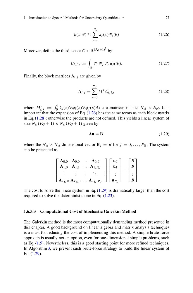
where the N el × N el dimensional vector B j = B for j = 0, . . . , P G . The system
can be presented as
⎡
⎢
⎢
⎢
⎣
A 0,0 A 0,0 . . . A 0,0
A 1,0 A 1,1 . . . A 1,P G
. . .
. . .
. . .
. . .
. . .
A P G ,0 A P G ,1 . . . A P G ,P G
⎤
⎥
⎥
⎥
⎦
⎡
⎢
⎢
⎢
⎣
u 0
u 1
. . .
u P G
⎤
⎥
⎥
⎥
⎦
=
⎡
⎢
⎢
⎢
⎣
B
B
. . .
B
⎤
⎥
⎥
⎥
⎦
The cost to solve the linear system in Eq. (1.29) is dramatically larger than the cost
required to solve the deterministic one in Eq. (1.23).
1.6.3.3 Computational Cost of Stochastic Galerkin Method
The Galerkin method is the most computationally demanding method presented in
this chapter. A good background on linear algebra and matrix analysis techniques
is a must for reducing the cost of implementing this method. A simple brute-force
approach is usually not an option, even for one-dimensional simple problems, such
as Eq. (1.5). Nevertheless, this is a good starting point for more refined techniques.
In Algorithm 3, we present such brute-force strategy to build the linear system of
Eq. (1.29).
27
k(x, θ) ≈
P G
s=0
k s (x)Ψ s (θ )
(1.26)
Moreover, define the third tensor C ∈ R (P G +1) 3 by
C i,j,s :=
Θ
Ψ i Ψ j Ψ s dμ(θ ).
(1.27)
Finally, the block matrices A i,j are given by
A i,j =
P G
s=0
M
s C i,j,s
(1.28)
where M s
i,j :=
1
0 k s (x)∇φ i (x)∇φ j (x)dx are matrices of size N el × N el . It is
important that the expansion of Eq. (1.26) has the same terms as each block matrix
in Eq. (1.28); otherwise the products are not defined. This yields a linear system of
size N el (P G + 1) × N el (P G + 1) given by
Au = B.
(1.29)
where the N el × N el dimensional vector B j = B for j = 0, . . . , P G . The system
can be presented as
⎡
⎢
⎢
⎢
⎣
A 0,0 A 0,0 . . . A 0,0
A 1,0 A 1,1 . . . A 1,P G
. . .
. . .
. . .
. . .
. . .
A P G ,0 A P G ,1 . . . A P G ,P G
⎤
⎥
⎥
⎥
⎦
⎡
⎢
⎢
⎢
⎣
u 0
u 1
. . .
u P G
⎤
⎥
⎥
⎥
⎦
=
⎡
⎢
⎢
⎢
⎣
B
B
. . .
B
⎤
⎥
⎥
⎥
⎦
The cost to solve the linear system in Eq. (1.29) is dramatically larger than the cost
required to solve the deterministic one in Eq. (1.23).
1.6.3.3 Computational Cost of Stochastic Galerkin Method
The Galerkin method is the most computationally demanding method presented in
this chapter. A good background on linear algebra and matrix analysis techniques
is a must for reducing the cost of implementing this method. A simple brute-force
approach is usually not an option, even for one-dimensional simple problems, such
as Eq. (1.5). Nevertheless, this is a good starting point for more refined techniques.
In Algorithm 3, we present such brute-force strategy to build the linear system of
Eq. (1.29).