

26
J. F. Reis et al.
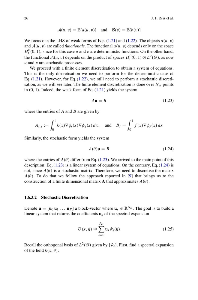
A(u, v) = E[a(u, v)] and B(v) = E[b(v)]
We focus one the LHS of weak forms of Eqs. (1.21) and (1.22). The objects a(u, v)
and A(u, v) are called functionals. The functional a(u, v) depends only on the space
H 0
1 (0, 1), since for this case u and v are deterministic functions. On the other hand,
the functional A(u, v) depends on the product of spaces H 0
1 (0, 1) ⊗ L 2 (Θ), as now
u and v are stochastic processes.
We proceed with a finite element discretisation to obtain a system of equations.
This is the only discretisation we need to perform for the deterministic case of
Eq. (1.21). However, for Eq. (1.22), we still need to perform a stochastic discretisation, as we will see later. The finite element discretisation is done over N el points
in (0, 1). Indeed, the weak form of Eq. (1.21) yields the system
Au = B
(1.23)
where the entries of A and B are given by
A i,j :=
1
0
k(x)∇φ i (x)∇φ j (x) dx, and B j =
1
0
f (x)∇φ j (x) dx
Similarly, the stochastic form yields the system
A(θ )u = B
(1.24)
where the entries of A(θ ) differ from Eq. (1.23). We arrived to the main point of this
description: Eq. (1.23) is a linear system of equations. On the contrary, Eq. (1.24) is
not, since A(θ ) is a stochastic matrix. Therefore, we need to discretise the matrix
A(θ ). To do that we follow the approach reported in [9] that brings us to the
construction of a finite dimensional matrix A that approximates A(θ ).
1.6.3.2 Stochastic Discretisation
Denote u = [u 0 u 1 . . . u P ] a block-vector where u s ∈ R N el . The goal is to build a
linear system that returns the coefficients u s of the spectral expansion
U(x, ξ ) ≈
P G
s=0
u s Ψ s (ξ )
(1.25)
Recall the orthogonal basis of L 2 (Θ) given by {Ψ s }. First, find a spectral expansion
of the field k(x, θ),
J. F. Reis et al.
A(u, v) = E[a(u, v)] and B(v) = E[b(v)]
We focus one the LHS of weak forms of Eqs. (1.21) and (1.22). The objects a(u, v)
and A(u, v) are called functionals. The functional a(u, v) depends only on the space
H 0
1 (0, 1), since for this case u and v are deterministic functions. On the other hand,
the functional A(u, v) depends on the product of spaces H 0
1 (0, 1) ⊗ L 2 (Θ), as now
u and v are stochastic processes.
We proceed with a finite element discretisation to obtain a system of equations.
This is the only discretisation we need to perform for the deterministic case of
Eq. (1.21). However, for Eq. (1.22), we still need to perform a stochastic discretisation, as we will see later. The finite element discretisation is done over N el points
in (0, 1). Indeed, the weak form of Eq. (1.21) yields the system
Au = B
(1.23)
where the entries of A and B are given by
A i,j :=
1
0
k(x)∇φ i (x)∇φ j (x) dx, and B j =
1
0
f (x)∇φ j (x) dx
Similarly, the stochastic form yields the system
A(θ )u = B
(1.24)
where the entries of A(θ ) differ from Eq. (1.23). We arrived to the main point of this
description: Eq. (1.23) is a linear system of equations. On the contrary, Eq. (1.24) is
not, since A(θ ) is a stochastic matrix. Therefore, we need to discretise the matrix
A(θ ). To do that we follow the approach reported in [9] that brings us to the
construction of a finite dimensional matrix A that approximates A(θ ).
1.6.3.2 Stochastic Discretisation
Denote u = [u 0 u 1 . . . u P ] a block-vector where u s ∈ R N el . The goal is to build a
linear system that returns the coefficients u s of the spectral expansion
U(x, ξ ) ≈
P G
s=0
u s Ψ s (ξ )
(1.25)
Recall the orthogonal basis of L 2 (Θ) given by {Ψ s }. First, find a spectral expansion
of the field k(x, θ),