

8 An Introduction to Many-Objective Evolutionary Optimization
297
uations. After the offspring are preselected, the optimizer continues as it would
normally. The algorithm is presented in Algorithm 6 [20].
Algorithm 6 Prescreening algorithm
t = 0
P (t) ← Initial population with size μ
Evaluate P (t) and database of evaluated points D
while Stopping criteria not fulfilled do
while |P (t)| < λ do
P (t) ← variation P (t)
Evaluate P (t) using surrogate model based on D
while |P (t)| < λ do
P (t) ← P
best (t), P
best (t) : member of P (t) with max improvement
P (t + 1) ← selection from Q ∪ P (t)
t = t + 1
8.5.3 Taxonomy of Surrogate Models for MOP
As we have seen above, introducing surrogate modelling to MOP can be done in
many ways. Deb et al. [14] classified the methods by how many surrogates are used
to treat the objectives and constraints. Deb classified them into six groups with the
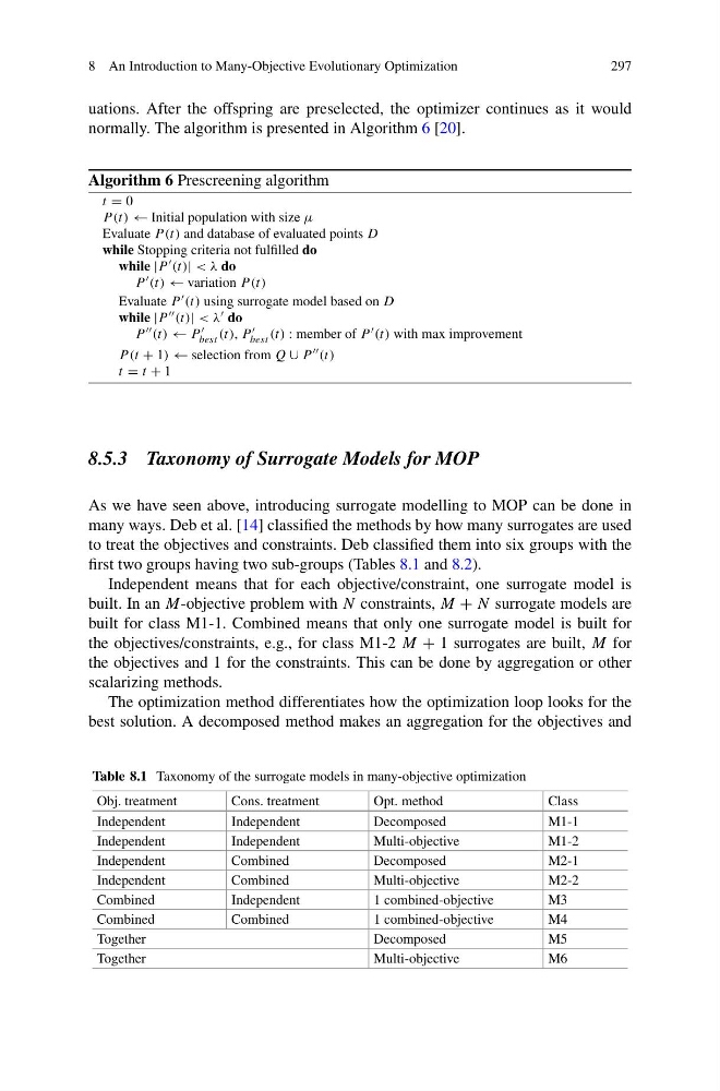
first two groups having two sub-groups (Tables 8.1 and 8.2).
Independent means that for each objective/constraint, one surrogate model is
built. In an M-objective problem with N constraints, M + N surrogate models are
built for class M1-1. Combined means that only one surrogate model is built for
the objectives/constraints, e.g., for class M1-2 M + 1 surrogates are built, M for
the objectives and 1 for the constraints. This can be done by aggregation or other
scalarizing methods.
The optimization method differentiates how the optimization loop looks for the
best solution. A decomposed method makes an aggregation for the objectives and
Table 8.1 Taxonomy of the surrogate models in many-objective optimization
Obj. treatment
Cons. treatment
Opt. method
Class
Independent
Independent
Decomposed
M1-1
Independent
Independent
Multi-objective
M1-2
Independent
Combined
Decomposed
M2-1
Independent
Combined
Multi-objective
M2-2
Combined
Independent
1 combined-objective
M3
Combined
Combined
1 combined-objective
M4
Together
Decomposed
M5
Together
Multi-objective
M6
297
uations. After the offspring are preselected, the optimizer continues as it would
normally. The algorithm is presented in Algorithm 6 [20].
Algorithm 6 Prescreening algorithm
t = 0
P (t) ← Initial population with size μ
Evaluate P (t) and database of evaluated points D
while Stopping criteria not fulfilled do
while |P (t)| < λ do
P (t) ← variation P (t)
Evaluate P (t) using surrogate model based on D
while |P (t)| < λ do
P (t) ← P
best (t), P
best (t) : member of P (t) with max improvement
P (t + 1) ← selection from Q ∪ P (t)
t = t + 1
8.5.3 Taxonomy of Surrogate Models for MOP
As we have seen above, introducing surrogate modelling to MOP can be done in
many ways. Deb et al. [14] classified the methods by how many surrogates are used
to treat the objectives and constraints. Deb classified them into six groups with the
first two groups having two sub-groups (Tables 8.1 and 8.2).
Independent means that for each objective/constraint, one surrogate model is
built. In an M-objective problem with N constraints, M + N surrogate models are
built for class M1-1. Combined means that only one surrogate model is built for
the objectives/constraints, e.g., for class M1-2 M + 1 surrogates are built, M for
the objectives and 1 for the constraints. This can be done by aggregation or other
scalarizing methods.
The optimization method differentiates how the optimization loop looks for the
best solution. A decomposed method makes an aggregation for the objectives and
Table 8.1 Taxonomy of the surrogate models in many-objective optimization
Obj. treatment
Cons. treatment
Opt. method
Class
Independent
Independent
Decomposed
M1-1
Independent
Independent
Multi-objective
M1-2
Independent
Combined
Decomposed
M2-1
Independent
Combined
Multi-objective
M2-2
Combined
Independent
1 combined-objective
M3
Combined
Combined
1 combined-objective
M4
Together
Decomposed
M5
Together
Multi-objective
M6