

1 Introduction to Spectral Methods for Uncertainty Quantification
17
equal to the number of elements employed, but it can be reduced if the field is
strongly correlated.
To apply the MC approach, the set of k i is sampled M times, according to its
KL parametrisation. For each m-th sample set, we deterministically compute the
value of temperature U (m) at a specific location, say at the beam mid-point. U (m)
is called the m-th realisation of the MC procedure. By the law of large numbers,
the M realisations can be used to compute the statistical moments of the solution
U . Obviously, from very few realisations, we cannot retrieve sufficient information
to compute statistical meaningful quantities. As we increase their number, we
extend the MC set and therefore improve the quantity of information available. In
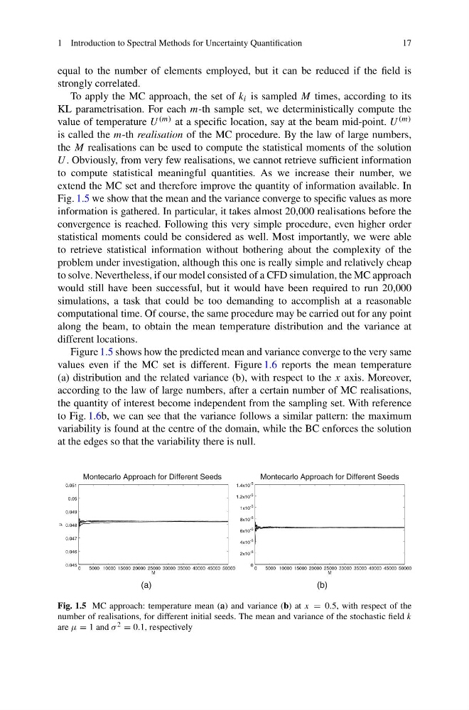
Fig. 1.5 we show that the mean and the variance converge to specific values as more
information is gathered. In particular, it takes almost 20,000 realisations before the
convergence is reached. Following this very simple procedure, even higher order
statistical moments could be considered as well. Most importantly, we were able
to retrieve statistical information without bothering about the complexity of the
problem under investigation, although this one is really simple and relatively cheap
to solve. Nevertheless, if our model consisted of a CFD simulation, the MC approach
would still have been successful, but it would have been required to run 20,000
simulations, a task that could be too demanding to accomplish at a reasonable
computational time. Of course, the same procedure may be carried out for any point
along the beam, to obtain the mean temperature distribution and the variance at
different locations.
Figure 1.5 shows how the predicted mean and variance converge to the very same
values even if the MC set is different. Figure 1.6 reports the mean temperature
(a) distribution and the related variance (b), with respect to the x axis. Moreover,
according to the law of large numbers, after a certain number of MC realisations,
the quantity of interest become independent from the sampling set. With reference
to Fig. 1.6b, we can see that the variance follows a similar pattern: the maximum
variability is found at the centre of the domain, while the BC enforces the solution
at the edges so that the variability there is null.
0.045
0.046
0.047
0.048
0.049
0.05
0.051
0
5000 10000 15000 20000 25000 30000 35000 40000 45000 50000
µ
M
Montecarlo Approach for Different Seeds
(a)
0
2x10 -6
4x10 -6
6x10 -6
8x10 -6
1x10 -5
1.2x10 -5
1.4x10 -5
0
5000 10000 15000 20000 25000 30000 35000 40000 45000 50000
M
Montecarlo Approach for Different Seeds
(b)
Fig. 1.5 MC approach: temperature mean (a) and variance (b) at x = 0.5, with respect of the
number of realisations, for different initial seeds. The mean and variance of the stochastic field k
are μ = 1 and σ 2 = 0.1, respectively
17
equal to the number of elements employed, but it can be reduced if the field is
strongly correlated.
To apply the MC approach, the set of k i is sampled M times, according to its
KL parametrisation. For each m-th sample set, we deterministically compute the
value of temperature U (m) at a specific location, say at the beam mid-point. U (m)
is called the m-th realisation of the MC procedure. By the law of large numbers,
the M realisations can be used to compute the statistical moments of the solution
U . Obviously, from very few realisations, we cannot retrieve sufficient information
to compute statistical meaningful quantities. As we increase their number, we
extend the MC set and therefore improve the quantity of information available. In
Fig. 1.5 we show that the mean and the variance converge to specific values as more
information is gathered. In particular, it takes almost 20,000 realisations before the
convergence is reached. Following this very simple procedure, even higher order
statistical moments could be considered as well. Most importantly, we were able
to retrieve statistical information without bothering about the complexity of the
problem under investigation, although this one is really simple and relatively cheap
to solve. Nevertheless, if our model consisted of a CFD simulation, the MC approach
would still have been successful, but it would have been required to run 20,000
simulations, a task that could be too demanding to accomplish at a reasonable
computational time. Of course, the same procedure may be carried out for any point
along the beam, to obtain the mean temperature distribution and the variance at
different locations.
Figure 1.5 shows how the predicted mean and variance converge to the very same
values even if the MC set is different. Figure 1.6 reports the mean temperature
(a) distribution and the related variance (b), with respect to the x axis. Moreover,
according to the law of large numbers, after a certain number of MC realisations,
the quantity of interest become independent from the sampling set. With reference
to Fig. 1.6b, we can see that the variance follows a similar pattern: the maximum
variability is found at the centre of the domain, while the BC enforces the solution
at the edges so that the variability there is null.
0.045
0.046
0.047
0.048
0.049
0.05
0.051
0
5000 10000 15000 20000 25000 30000 35000 40000 45000 50000
µ
M
Montecarlo Approach for Different Seeds
(a)
0
2x10 -6
4x10 -6
6x10 -6
8x10 -6
1x10 -5
1.2x10 -5
1.4x10 -5
0
5000 10000 15000 20000 25000 30000 35000 40000 45000 50000
M
Montecarlo Approach for Different Seeds
(b)
Fig. 1.5 MC approach: temperature mean (a) and variance (b) at x = 0.5, with respect of the
number of realisations, for different initial seeds. The mean and variance of the stochastic field k
are μ = 1 and σ 2 = 0.1, respectively