

212
C. Greco and M. Vasile
P
+
k = P
−
k − K k S k K
T
k .
(6.83)
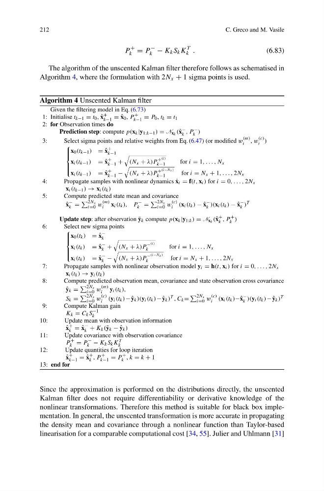
The algorithm of the unscented Kalman filter therefore follows as schematised in
Algorithm 4, where the formulation with 2N x + 1 sigma points is used.
Algorithm 4 Unscented Kalman filter
Given the filtering model in Eq. (6.73)
1: Initialise t k−1 = t 0 , ˆ
x
+
k−1 = ˆ
x 0 , P
+
k−1 = P 0 , t k = t 1
2: for Observation times do
Prediction step: compute p(x k |y 1:k−1 ) = N x k (ˆ x
−
k , P
−
k )
3:
Select sigma points and relative weights from Eq. (6.47) (or modified w
(m)
i , w
(c)
i )
⎧
⎪ ⎪ ⎨
⎪ ⎪ ⎩
x 0 (t k−1 ) = ˆ
x
+
k−1
x i (t k−1 ) = ˆ
x
+
k−1 +
(N x + λ)P
+ (i)
k−1
for i = 1, . . . , N x
x i (t k−1 ) = ˆ
x
+
k−1 −
(N x + λ)P
+ (i−Nx )
k−1
for i = N x + 1, . . . , 2N x
4:
Propagate samples with nonlinear dynamics ˙
x i = f(t, x i ) for i = 0, . . . , 2N x
x i (t k−1 ) → x i (t k )
5:
Compute predicted state mean and covariance
ˆ
x
−
k =
2Nx
i=0 w
(m)
i
x i (t k ), P
−
k =
2Nx
i=0 w
(c)
i (x i (t k ) − ˆ
x
−
k )(x i (t k ) − ˆ
x
−
k ) T
Update step: after observation ¯
y k compute p(x k |y 1:k ) = N x k (ˆ x
+
k , P
+
k )
6:
Select new sigma points
⎧
⎪ ⎪ ⎨
⎪ ⎪ ⎩
x 0 (t k ) = ˆ
x
−
k
x i (t k ) = ˆ
x
−
k +
(N x + λ)P
− (i)
k
for i = 1, . . . , N x
x i (t k ) = ˆ
x
−
k −
(N x + λ)P
− (i−Nx )
k
for i = N x + 1, . . . , 2N x
7:
Propagate samples with nonlinear observation model y i = h(t, x i ) for i = 0, . . . , 2N x
x i (t k ) → y i (t k )
8:
Compute predicted observation mean, covariance and state observation cross covariance
ˆ
y k =
2Nx
i=0 w
(m)
i
y i (t k ),
S k =
2Nx
i=0 w
(c)
i (y i (t k )− ˆ
y k )(y i (t k )− ˆ
y k ) T , C k =
2Nx
i=0 w
(c)
i (x i (t k )−ˆ x
−
k )(y i (t k )− ˆ
y k ) T
9:
Compute Kalman gain
K k = C k S
−1
k
10:
Update mean with observation information
ˆ
x
+
k = ˆ
x
−
k + K k (¯ y k − ˆ
y k )
11:
Update covariance with observation covariance
P
+
k = P
−
k − K k S k K T
k
12:
Update quantities for loop iteration
ˆ
x
+
k−1 = ˆ
x
+
k , P
+
k−1 = P
+
k , k = k + 1
13: end for
Since the approximation is performed on the distributions directly, the unscented
Kalman filter does not require differentiability or derivative knowledge of the
nonlinear transformations. Therefore this method is suitable for black box implementation. In general, the unscented transformation is more accurate in propagating
the density mean and covariance through a nonlinear function than Taylor-based
linearisation for a comparable computational cost [34, 55]. Julier and Uhlmann [31]
C. Greco and M. Vasile
P
+
k = P
−
k − K k S k K
T
k .
(6.83)
The algorithm of the unscented Kalman filter therefore follows as schematised in
Algorithm 4, where the formulation with 2N x + 1 sigma points is used.
Algorithm 4 Unscented Kalman filter
Given the filtering model in Eq. (6.73)
1: Initialise t k−1 = t 0 , ˆ
x
+
k−1 = ˆ
x 0 , P
+
k−1 = P 0 , t k = t 1
2: for Observation times do
Prediction step: compute p(x k |y 1:k−1 ) = N x k (ˆ x
−
k , P
−
k )
3:
Select sigma points and relative weights from Eq. (6.47) (or modified w
(m)
i , w
(c)
i )
⎧
⎪ ⎪ ⎨
⎪ ⎪ ⎩
x 0 (t k−1 ) = ˆ
x
+
k−1
x i (t k−1 ) = ˆ
x
+
k−1 +
(N x + λ)P
+ (i)
k−1
for i = 1, . . . , N x
x i (t k−1 ) = ˆ
x
+
k−1 −
(N x + λ)P
+ (i−Nx )
k−1
for i = N x + 1, . . . , 2N x
4:
Propagate samples with nonlinear dynamics ˙
x i = f(t, x i ) for i = 0, . . . , 2N x
x i (t k−1 ) → x i (t k )
5:
Compute predicted state mean and covariance
ˆ
x
−
k =
2Nx
i=0 w
(m)
i
x i (t k ), P
−
k =
2Nx
i=0 w
(c)
i (x i (t k ) − ˆ
x
−
k )(x i (t k ) − ˆ
x
−
k ) T
Update step: after observation ¯
y k compute p(x k |y 1:k ) = N x k (ˆ x
+
k , P
+
k )
6:
Select new sigma points
⎧
⎪ ⎪ ⎨
⎪ ⎪ ⎩
x 0 (t k ) = ˆ
x
−
k
x i (t k ) = ˆ
x
−
k +
(N x + λ)P
− (i)
k
for i = 1, . . . , N x
x i (t k ) = ˆ
x
−
k −
(N x + λ)P
− (i−Nx )
k
for i = N x + 1, . . . , 2N x
7:
Propagate samples with nonlinear observation model y i = h(t, x i ) for i = 0, . . . , 2N x
x i (t k ) → y i (t k )
8:
Compute predicted observation mean, covariance and state observation cross covariance
ˆ
y k =
2Nx
i=0 w
(m)
i
y i (t k ),
S k =
2Nx
i=0 w
(c)
i (y i (t k )− ˆ
y k )(y i (t k )− ˆ
y k ) T , C k =
2Nx
i=0 w
(c)
i (x i (t k )−ˆ x
−
k )(y i (t k )− ˆ
y k ) T
9:
Compute Kalman gain
K k = C k S
−1
k
10:
Update mean with observation information
ˆ
x
+
k = ˆ
x
−
k + K k (¯ y k − ˆ
y k )
11:
Update covariance with observation covariance
P
+
k = P
−
k − K k S k K T
k
12:
Update quantities for loop iteration
ˆ
x
+
k−1 = ˆ
x
+
k , P
+
k−1 = P
+
k , k = k + 1
13: end for
Since the approximation is performed on the distributions directly, the unscented
Kalman filter does not require differentiability or derivative knowledge of the
nonlinear transformations. Therefore this method is suitable for black box implementation. In general, the unscented transformation is more accurate in propagating
the density mean and covariance through a nonlinear function than Taylor-based
linearisation for a comparable computational cost [34, 55]. Julier and Uhlmann [31]