

6 Fundamentals of Filtering
211
6.3.3 Unscented Kalman Filter
The unscented Kalman filter (UKF) works directly with the nonlinear filtering
model, i.e. without approximating the nonlinear transformations. Hence, the derivation presented for the Kalman filter and adapted for the extended version needs to
be updated for nonlinear functions.
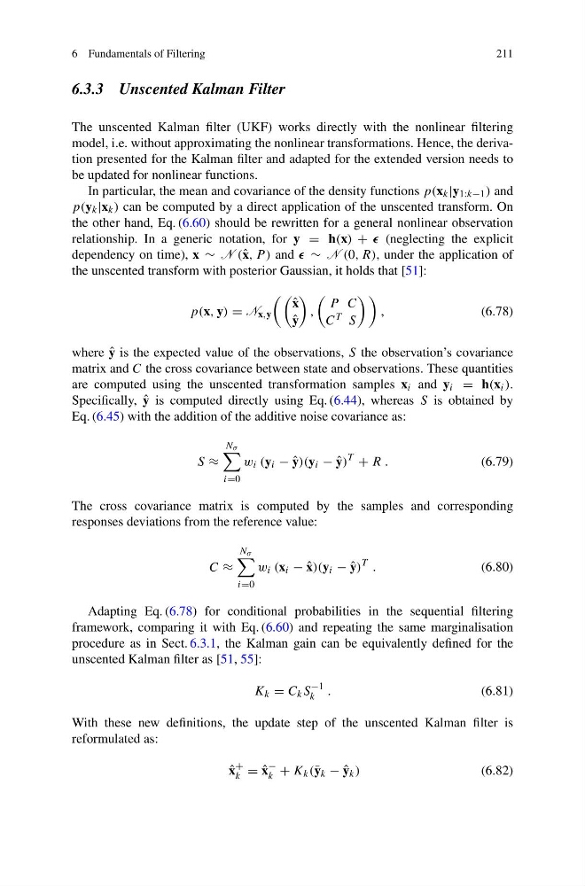
In particular, the mean and covariance of the density functions p(x k |y 1:k−1 ) and
p(y k |x k ) can be computed by a direct application of the unscented transform. On
the other hand, Eq. (6.60) should be rewritten for a general nonlinear observation
relationship. In a generic notation, for y = h(x) + (neglecting the explicit
dependency on time), x ∼ N (ˆ x, P ) and ∼ N (0, R), under the application of
the unscented transform with posterior Gaussian, it holds that [51]:
p(x, y) = N x,y
ˆ
x
ˆ
y
,
P C
C T S
,
(6.78)
where ˆ
y is the expected value of the observations, S the observation’s covariance
matrix and C the cross covariance between state and observations. These quantities
are computed using the unscented transformation samples x i and y i = h(x i ).
Specifically, ˆ
y is computed directly using Eq. (6.44), whereas S is obtained by
Eq. (6.45) with the addition of the additive noise covariance as:
S ≈
N σ
i=0
w i (y i − ˆ
y)(y i − ˆ
y)
T
+ R .
(6.79)
The cross covariance matrix is computed by the samples and corresponding
responses deviations from the reference value:
C ≈
N σ
i=0
w i (x i − ˆ
x)(y i − ˆ
y)
T .
(6.80)
Adapting Eq. (6.78) for conditional probabilities in the sequential filtering
framework, comparing it with Eq. (6.60) and repeating the same marginalisation
procedure as in Sect. 6.3.1, the Kalman gain can be equivalently defined for the
unscented Kalman filter as [51, 55]:
K k = C k S
−1
k .
(6.81)
With these new definitions, the update step of the unscented Kalman filter is
reformulated as:
ˆ
x
+
k = ˆ
x
−
k + K k (¯ y k − ˆ
y k )
(6.82)
211
6.3.3 Unscented Kalman Filter
The unscented Kalman filter (UKF) works directly with the nonlinear filtering
model, i.e. without approximating the nonlinear transformations. Hence, the derivation presented for the Kalman filter and adapted for the extended version needs to
be updated for nonlinear functions.
In particular, the mean and covariance of the density functions p(x k |y 1:k−1 ) and
p(y k |x k ) can be computed by a direct application of the unscented transform. On
the other hand, Eq. (6.60) should be rewritten for a general nonlinear observation
relationship. In a generic notation, for y = h(x) + (neglecting the explicit
dependency on time), x ∼ N (ˆ x, P ) and ∼ N (0, R), under the application of
the unscented transform with posterior Gaussian, it holds that [51]:
p(x, y) = N x,y
ˆ
x
ˆ
y
,
P C
C T S
,
(6.78)
where ˆ
y is the expected value of the observations, S the observation’s covariance
matrix and C the cross covariance between state and observations. These quantities
are computed using the unscented transformation samples x i and y i = h(x i ).
Specifically, ˆ
y is computed directly using Eq. (6.44), whereas S is obtained by
Eq. (6.45) with the addition of the additive noise covariance as:
S ≈
N σ
i=0
w i (y i − ˆ
y)(y i − ˆ
y)
T
+ R .
(6.79)
The cross covariance matrix is computed by the samples and corresponding
responses deviations from the reference value:
C ≈
N σ
i=0
w i (x i − ˆ
x)(y i − ˆ
y)
T .
(6.80)
Adapting Eq. (6.78) for conditional probabilities in the sequential filtering
framework, comparing it with Eq. (6.60) and repeating the same marginalisation
procedure as in Sect. 6.3.1, the Kalman gain can be equivalently defined for the
unscented Kalman filter as [51, 55]:
K k = C k S
−1
k .
(6.81)
With these new definitions, the update step of the unscented Kalman filter is
reformulated as:
ˆ
x
+
k = ˆ
x
−
k + K k (¯ y k − ˆ
y k )
(6.82)