

196
C. Greco and M. Vasile
z = g(x) = g(ˆ x) + ∇ x g
ˆ
x
(x − ˆ
x) +
1
2
i
(x − ˆ
x)
T H
(i)
xx
ˆ
x
(x − ˆ
x)e i + O
(x − ˆ
x)
3
,
(6.39)
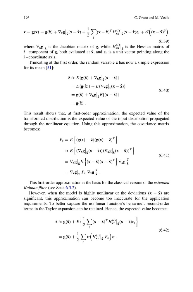
where ∇ x g
ˆ
x
is the Jacobian matrix of g, while H
(i)
xx
ˆ
x
is the Hessian matrix of
i−component of g, both evaluated at ˆ
x, and e i is a unit vector pointing along the
i−coordinate axis.
Truncating at the first order, the random variable z has now a simple expression
for its mean [51]:
ˆ
z ≈ E{g(ˆ x) + ∇ x g
ˆ
x
(x − ˆ
x)}
= E{g(ˆ x)} + E{∇ x g
ˆ
x
(x − ˆ
x)}
= g(ˆ x) + ∇ x g
ˆ
x
E{(x − ˆ
x)}
= g(ˆ x) .
(6.40)
This result shows that, at first-order approximation, the expected value of the
transformed distribution is the expected value of the input distribution propagated
through the nonlinear equation. Using this approximation, the covariance matrix
becomes:
P z = E
(g(x) − ˆ
z)(g(x) − ˆ
z)
T
≈ E
(∇ x g
ˆ
x
(x − ˆ
x))(∇ x g
ˆ
x
(x − ˆ
x))
T
= ∇ x g
ˆ
x
E
(x − ˆ
x)(x − ˆ
x)
T
∇ x g
T
ˆ
x
= ∇ x g
ˆ
x
P x ∇ x g
T
ˆ
x
.
(6.41)
This first-order approximation is the basis for the classical version of the extended
Kalman filter (see Sect. 6.3.2).
However, when the model is highly nonlinear or the deviations (x − ˆ
x) are
significant, this approximation can become too inaccurate for the application
requirements. To better capture the nonlinear function’s behaviour, second-order
terms in the Taylor expansion can be retained. Hence, the expected value becomes:
ˆ
z ≈ g(ˆ x) + E
1
2
i
(x − ˆ
x)
T H
(i)
xx
ˆ
x
(x − ˆ
x)e i
= g(ˆ x) +
1
2
i
tr
H
(i)
xx
ˆ
x
P x
e i .
(6.42)
C. Greco and M. Vasile
z = g(x) = g(ˆ x) + ∇ x g
ˆ
x
(x − ˆ
x) +
1
2
i
(x − ˆ
x)
T H
(i)
xx
ˆ
x
(x − ˆ
x)e i + O
(x − ˆ
x)
3
,
(6.39)
where ∇ x g
ˆ
x
is the Jacobian matrix of g, while H
(i)
xx
ˆ
x
is the Hessian matrix of
i−component of g, both evaluated at ˆ
x, and e i is a unit vector pointing along the
i−coordinate axis.
Truncating at the first order, the random variable z has now a simple expression
for its mean [51]:
ˆ
z ≈ E{g(ˆ x) + ∇ x g
ˆ
x
(x − ˆ
x)}
= E{g(ˆ x)} + E{∇ x g
ˆ
x
(x − ˆ
x)}
= g(ˆ x) + ∇ x g
ˆ
x
E{(x − ˆ
x)}
= g(ˆ x) .
(6.40)
This result shows that, at first-order approximation, the expected value of the
transformed distribution is the expected value of the input distribution propagated
through the nonlinear equation. Using this approximation, the covariance matrix
becomes:
P z = E
(g(x) − ˆ
z)(g(x) − ˆ
z)
T
≈ E
(∇ x g
ˆ
x
(x − ˆ
x))(∇ x g
ˆ
x
(x − ˆ
x))
T
= ∇ x g
ˆ
x
E
(x − ˆ
x)(x − ˆ
x)
T
∇ x g
T
ˆ
x
= ∇ x g
ˆ
x
P x ∇ x g
T
ˆ
x
.
(6.41)
This first-order approximation is the basis for the classical version of the extended
Kalman filter (see Sect. 6.3.2).
However, when the model is highly nonlinear or the deviations (x − ˆ
x) are
significant, this approximation can become too inaccurate for the application
requirements. To better capture the nonlinear function’s behaviour, second-order
terms in the Taylor expansion can be retained. Hence, the expected value becomes:
ˆ
z ≈ g(ˆ x) + E
1
2
i
(x − ˆ
x)
T H
(i)
xx
ˆ
x
(x − ˆ
x)e i
= g(ˆ x) +
1
2
i
tr
H
(i)
xx
ˆ
x
P x
e i .
(6.42)