

1 Introduction to Spectral Methods for Uncertainty Quantification
13
0
0.2
0.4
0.6
0.8
1
1
2
3
4
5
6
7
8
9
10
l = 0.016
l = 0.08
l = 0.4
l = 2
l = 10
i /
max
Eigenvalue Index
KL Eigenvalues
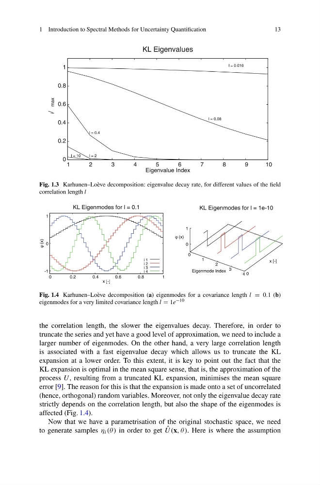
Fig. 1.3 Karhunen–Loève decomposition: eigenvalue decay rate, for different values of the field
correlation length l
-1
0
1
0
0.2
0.4
0.6
0.8
1
φ (x)
x [-]
KL Eigenmodes for l = 0.1
i 1
i 2
i 3
i 4
0
1
2
3
4 0
0
1
KL Eigenmodes for l = 1e-10
Eigenmode Index
x [-]
φ (x)
Fig. 1.4 Karhunen–Loève decomposition (a) eigenmodes for a covariance length l = 0.1 (b)
eigenmodes for a very limited covariance length l = 1e −10
the correlation length, the slower the eigenvalues decay. Therefore, in order to
truncate the series and yet have a good level of approximation, we need to include a
larger number of eigenmodes. On the other hand, a very large correlation length
is associated with a fast eigenvalue decay which allows us to truncate the KL
expansion at a lower order. To this extent, it is key to point out the fact that the
KL expansion is optimal in the mean square sense, that is, the approximation of the
process U , resulting from a truncated KL expansion, minimises the mean square
error [9]. The reason for this is that the expansion is made onto a set of uncorrelated
(hence, orthogonal) random variables. Moreover, not only the eigenvalue decay rate
strictly depends on the correlation length, but also the shape of the eigenmodes is
affected (Fig. 1.4).
Now that we have a parametrisation of the original stochastic space, we need
to generate samples η i (θ ) in order to get ˆ
U(x, θ). Here is where the assumption
13
0
0.2
0.4
0.6
0.8
1
1
2
3
4
5
6
7
8
9
10
l = 0.016
l = 0.08
l = 0.4
l = 2
l = 10
i /
max
Eigenvalue Index
KL Eigenvalues
Fig. 1.3 Karhunen–Loève decomposition: eigenvalue decay rate, for different values of the field
correlation length l
-1
0
1
0
0.2
0.4
0.6
0.8
1
φ (x)
x [-]
KL Eigenmodes for l = 0.1
i 1
i 2
i 3
i 4
0
1
2
3
4 0
0
1
KL Eigenmodes for l = 1e-10
Eigenmode Index
x [-]
φ (x)
Fig. 1.4 Karhunen–Loève decomposition (a) eigenmodes for a covariance length l = 0.1 (b)
eigenmodes for a very limited covariance length l = 1e −10
the correlation length, the slower the eigenvalues decay. Therefore, in order to
truncate the series and yet have a good level of approximation, we need to include a
larger number of eigenmodes. On the other hand, a very large correlation length
is associated with a fast eigenvalue decay which allows us to truncate the KL
expansion at a lower order. To this extent, it is key to point out the fact that the
KL expansion is optimal in the mean square sense, that is, the approximation of the
process U , resulting from a truncated KL expansion, minimises the mean square
error [9]. The reason for this is that the expansion is made onto a set of uncorrelated
(hence, orthogonal) random variables. Moreover, not only the eigenvalue decay rate
strictly depends on the correlation length, but also the shape of the eigenmodes is
affected (Fig. 1.4).
Now that we have a parametrisation of the original stochastic space, we need
to generate samples η i (θ ) in order to get ˆ
U(x, θ). Here is where the assumption