

5 An Introduction to Imprecise Markov Chains
153
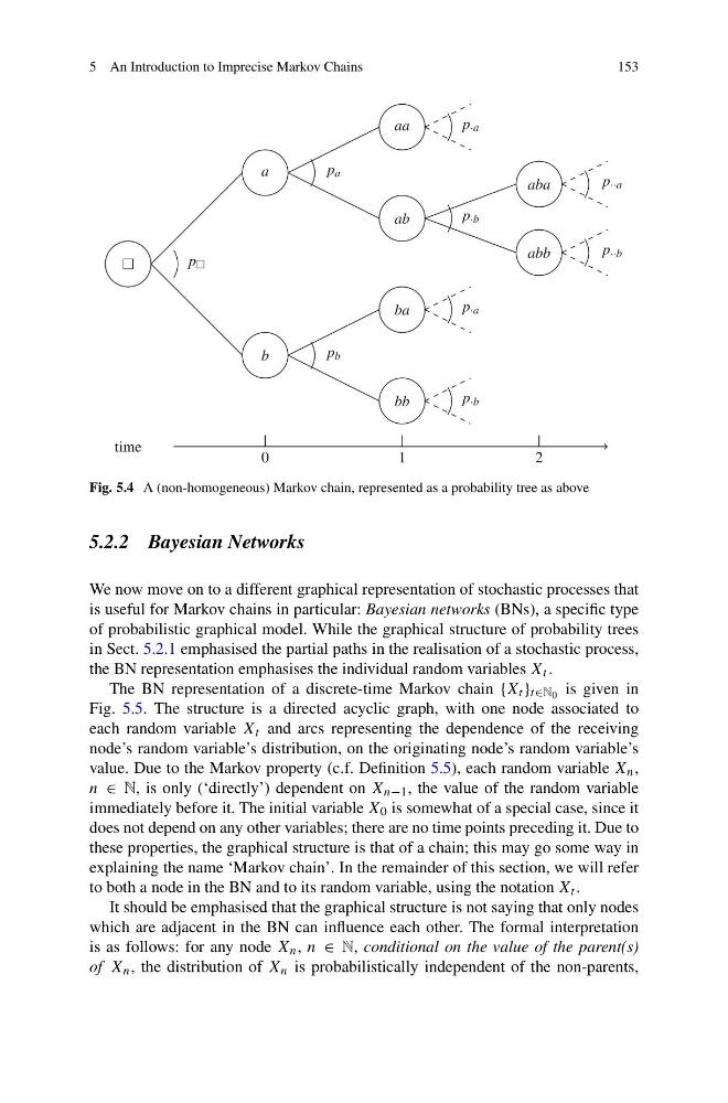
Fig. 5.4 A (non-homogeneous) Markov chain, represented as a probability tree as above
5.2.2 Bayesian Networks
We now move on to a different graphical representation of stochastic processes that
is useful for Markov chains in particular: Bayesian networks (BNs), a specific type
of probabilistic graphical model. While the graphical structure of probability trees
in Sect. 5.2.1 emphasised the partial paths in the realisation of a stochastic process,
the BN representation emphasises the individual random variables X t .
The BN representation of a discrete-time Markov chain {X t } t∈N 0 is given in
Fig. 5.5. The structure is a directed acyclic graph, with one node associated to
each random variable X t and arcs representing the dependence of the receiving
node’s random variable’s distribution, on the originating node’s random variable’s
value. Due to the Markov property (c.f. Definition 5.5), each random variable X n ,
n ∈ N, is only (‘directly’) dependent on X n−1 , the value of the random variable
immediately before it. The initial variable X 0 is somewhat of a special case, since it
does not depend on any other variables; there are no time points preceding it. Due to
these properties, the graphical structure is that of a chain; this may go some way in
explaining the name ‘Markov chain’. In the remainder of this section, we will refer
to both a node in the BN and to its random variable, using the notation X t .
It should be emphasised that the graphical structure is not saying that only nodes
which are adjacent in the BN can influence each other. The formal interpretation
is as follows: for any node X n , n ∈ N, conditional on the value of the parent(s)
of X n , the distribution of X n is probabilistically independent of the non-parents,
153
Fig. 5.4 A (non-homogeneous) Markov chain, represented as a probability tree as above
5.2.2 Bayesian Networks
We now move on to a different graphical representation of stochastic processes that
is useful for Markov chains in particular: Bayesian networks (BNs), a specific type
of probabilistic graphical model. While the graphical structure of probability trees
in Sect. 5.2.1 emphasised the partial paths in the realisation of a stochastic process,
the BN representation emphasises the individual random variables X t .
The BN representation of a discrete-time Markov chain {X t } t∈N 0 is given in
Fig. 5.5. The structure is a directed acyclic graph, with one node associated to
each random variable X t and arcs representing the dependence of the receiving
node’s random variable’s distribution, on the originating node’s random variable’s
value. Due to the Markov property (c.f. Definition 5.5), each random variable X n ,
n ∈ N, is only (‘directly’) dependent on X n−1 , the value of the random variable
immediately before it. The initial variable X 0 is somewhat of a special case, since it
does not depend on any other variables; there are no time points preceding it. Due to
these properties, the graphical structure is that of a chain; this may go some way in
explaining the name ‘Markov chain’. In the remainder of this section, we will refer
to both a node in the BN and to its random variable, using the notation X t .
It should be emphasised that the graphical structure is not saying that only nodes
which are adjacent in the BN can influence each other. The formal interpretation
is as follows: for any node X n , n ∈ N, conditional on the value of the parent(s)
of X n , the distribution of X n is probabilistically independent of the non-parents,