

6
J. F. Reis et al.
Hereafter, we will look for the steady solution of the heat diffusion problem only,
which in fact corresponds to the stable equilibrium state that is necessarily reached
after a sufficient amount of time.
This implies that we will consider the steady problem only, i.e. the system is nontransient, and the distribution of temperature does not depend on time. Moreover,
we will assume that the source term is constant in time and homogeneous in space
˙
q(x, t) = f . Under these hypotheses, the heat diffusion problem reduces to
∂ x k(x)∂ x u(x) = −f x ∈ (0, 1)
(1.2)
Throughout this chapter, we will compute the solution of this differential equation,
using a finite element method based on the Galerkin approach; see [4]. We therefore
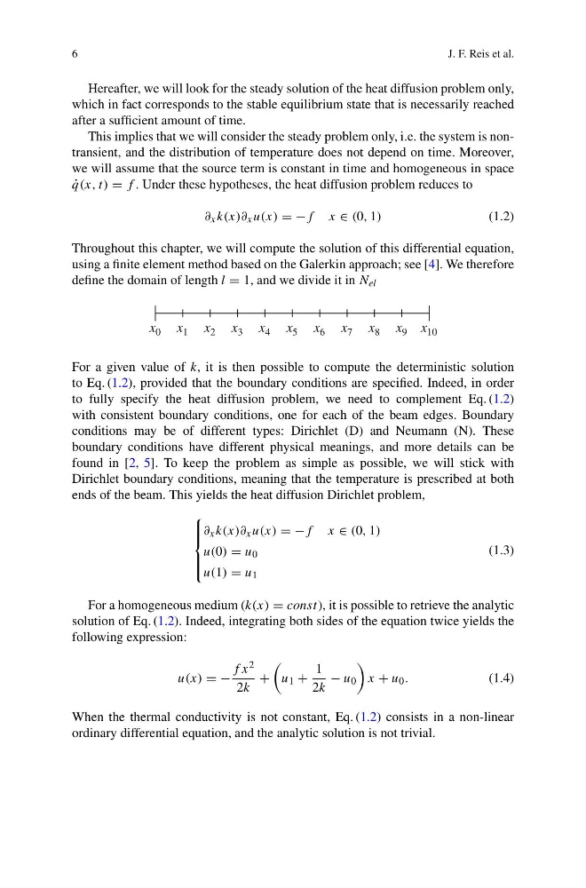
define the domain of length l = 1, and we divide it in N el
x 0 x 1 x 2 x 3 x 4 x 5 x 6 x 7 x 8 x 9 x 10
For a given value of k, it is then possible to compute the deterministic solution
to Eq. (1.2), provided that the boundary conditions are specified. Indeed, in order
to fully specify the heat diffusion problem, we need to complement Eq. (1.2)
with consistent boundary conditions, one for each of the beam edges. Boundary
conditions may be of different types: Dirichlet (D) and Neumann (N). These
boundary conditions have different physical meanings, and more details can be
found in [2, 5]. To keep the problem as simple as possible, we will stick with
Dirichlet boundary conditions, meaning that the temperature is prescribed at both
ends of the beam. This yields the heat diffusion Dirichlet problem,
⎧
⎪ ⎪ ⎨
⎪ ⎪ ⎩
∂ x k(x)∂ x u(x) = −f x ∈ (0, 1)
u(0) = u 0
u(1) = u 1
(1.3)
For a homogeneous medium (k(x) = const), it is possible to retrieve the analytic
solution of Eq. (1.2). Indeed, integrating both sides of the equation twice yields the
following expression:
u(x) = −
f x 2
2k
+
u 1 +
1
2k
− u 0
x + u 0 .
(1.4)
When the thermal conductivity is not constant, Eq. (1.2) consists in a non-linear
ordinary differential equation, and the analytic solution is not trivial.
J. F. Reis et al.
Hereafter, we will look for the steady solution of the heat diffusion problem only,
which in fact corresponds to the stable equilibrium state that is necessarily reached
after a sufficient amount of time.
This implies that we will consider the steady problem only, i.e. the system is nontransient, and the distribution of temperature does not depend on time. Moreover,
we will assume that the source term is constant in time and homogeneous in space
˙
q(x, t) = f . Under these hypotheses, the heat diffusion problem reduces to
∂ x k(x)∂ x u(x) = −f x ∈ (0, 1)
(1.2)
Throughout this chapter, we will compute the solution of this differential equation,
using a finite element method based on the Galerkin approach; see [4]. We therefore
define the domain of length l = 1, and we divide it in N el
x 0 x 1 x 2 x 3 x 4 x 5 x 6 x 7 x 8 x 9 x 10
For a given value of k, it is then possible to compute the deterministic solution
to Eq. (1.2), provided that the boundary conditions are specified. Indeed, in order
to fully specify the heat diffusion problem, we need to complement Eq. (1.2)
with consistent boundary conditions, one for each of the beam edges. Boundary
conditions may be of different types: Dirichlet (D) and Neumann (N). These
boundary conditions have different physical meanings, and more details can be
found in [2, 5]. To keep the problem as simple as possible, we will stick with
Dirichlet boundary conditions, meaning that the temperature is prescribed at both
ends of the beam. This yields the heat diffusion Dirichlet problem,
⎧
⎪ ⎪ ⎨
⎪ ⎪ ⎩
∂ x k(x)∂ x u(x) = −f x ∈ (0, 1)
u(0) = u 0
u(1) = u 1
(1.3)
For a homogeneous medium (k(x) = const), it is possible to retrieve the analytic
solution of Eq. (1.2). Indeed, integrating both sides of the equation twice yields the
following expression:
u(x) = −
f x 2
2k
+
u 1 +
1
2k
− u 0
x + u 0 .
(1.4)
When the thermal conductivity is not constant, Eq. (1.2) consists in a non-linear
ordinary differential equation, and the analytic solution is not trivial.