

100
T. Basu et al.
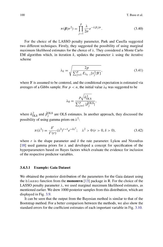
π(β|σ
2 ) =
p
j =1
λ
2σ
e
−λ|β j |σ .
(3.40)
For the choice of the LASSO penalty parameter, Park and Casella suggested
two different techniques. Firstly, they suggested the possibility of using marginal
maximum likelihood estimates for the choice of λ. They considered a Monte Carlo
EM algorithm which, in iteration k, updates the parameter λ using the iterative
scheme
λ k =
2p
p
j =1 E λ k−1 [τ 2
j |Y ]
,
(3.41)
where Y is assumed to be centered, and the conditional expectation is estimated via
averages of a Gibbs sample. For p < n, the initial value λ 0 was suggested to be
λ 0 =
p
ˆ
σ 2
OLS
p
j =1 | ˆ
β OLS
j
|
,
where ˆ
σ 2
OLS and ˆ
β OLS
j
are OLS estimates. In another approach, they discussed the
possibility of using gamma priors on λ 2 :
π(λ
2 ) =
δ r
Γ (r)
(λ
2 )
r−1 e
−δλ 2 ; λ
2 > 0 (r > 0, δ > 0),
(3.42)
where r is the shape parameter and δ the rate parameter. Lykou and Ntzoufras
[18] used gamma priors for λ and developed a concept for specification of the
hyperparameters based on Bayes factors which evaluate the evidence for inclusion
of the respective predictor variables.
3.4.3.1 Example: Gaia Dataset
We obtained the posterior distribution of the parameters for the Gaia dataset using
the blasso function from the monomvn [13] package in R. For the choice of the
LASSO penalty parameter λ, we used marginal maximum likelihood estimates, as
mentioned earlier. We drew 1000 posterior samples from this distribution, which are
displayed in Fig. 3.9.
It can be seen that the output from the Bayesian method is similar to that of the
Bootstrap method. For a better comparison between the methods, we also show the
standard errors for the coefficient estimates of each important variable in Fig. 3.10.
T. Basu et al.
π(β|σ
2 ) =
p
j =1
λ
2σ
e
−λ|β j |σ .
(3.40)
For the choice of the LASSO penalty parameter, Park and Casella suggested
two different techniques. Firstly, they suggested the possibility of using marginal
maximum likelihood estimates for the choice of λ. They considered a Monte Carlo
EM algorithm which, in iteration k, updates the parameter λ using the iterative
scheme
λ k =
2p
p
j =1 E λ k−1 [τ 2
j |Y ]
,
(3.41)
where Y is assumed to be centered, and the conditional expectation is estimated via
averages of a Gibbs sample. For p < n, the initial value λ 0 was suggested to be
λ 0 =
p
ˆ
σ 2
OLS
p
j =1 | ˆ
β OLS
j
|
,
where ˆ
σ 2
OLS and ˆ
β OLS
j
are OLS estimates. In another approach, they discussed the
possibility of using gamma priors on λ 2 :
π(λ
2 ) =
δ r
Γ (r)
(λ
2 )
r−1 e
−δλ 2 ; λ
2 > 0 (r > 0, δ > 0),
(3.42)
where r is the shape parameter and δ the rate parameter. Lykou and Ntzoufras
[18] used gamma priors for λ and developed a concept for specification of the
hyperparameters based on Bayes factors which evaluate the evidence for inclusion
of the respective predictor variables.
3.4.3.1 Example: Gaia Dataset
We obtained the posterior distribution of the parameters for the Gaia dataset using
the blasso function from the monomvn [13] package in R. For the choice of the
LASSO penalty parameter λ, we used marginal maximum likelihood estimates, as
mentioned earlier. We drew 1000 posterior samples from this distribution, which are
displayed in Fig. 3.9.
It can be seen that the output from the Bayesian method is similar to that of the
Bootstrap method. For a better comparison between the methods, we also show the
standard errors for the coefficient estimates of each important variable in Fig. 3.10.