

3 Uncertainty Quantification in Lasso-Type Regularization Problems
99
3.4.3 Bayesian LASSO
The Bayesian methodology provides a natural way to quantify the model uncertainty
in a LASSO-fitted model. To motivate this approach, recall firstly that, under the
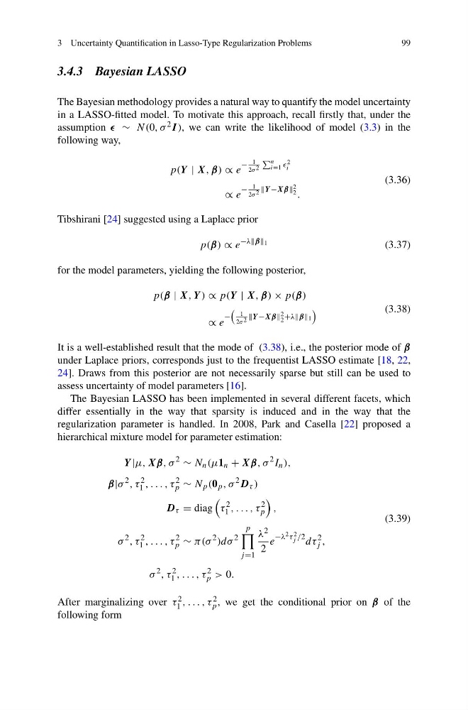
assumption ∼ N(0, σ 2 I ), we can write the likelihood of model (3.3) in the
following way,
p(Y | X, β) ∝ e
−
1
2σ 2
n
i=1 2
i
∝ e
−
1
2σ 2 Y −Xβ 2
2 .
(3.36)
Tibshirani [24] suggested using a Laplace prior
p(β) ∝ e
−λβ 1
(3.37)
for the model parameters, yielding the following posterior,
p(β | X, Y ) ∝ p(Y | X, β) × p(β)
∝ e
−
1
2σ 2 Y −Xβ 2
2 +λβ 1
(3.38)
It is a well-established result that the mode of (3.38), i.e., the posterior mode of β
under Laplace priors, corresponds just to the frequentist LASSO estimate [18, 22,
24]. Draws from this posterior are not necessarily sparse but still can be used to
assess uncertainty of model parameters [16].
The Bayesian LASSO has been implemented in several different facets, which
differ essentially in the way that sparsity is induced and in the way that the
regularization parameter is handled. In 2008, Park and Casella [22] proposed a
hierarchical mixture model for parameter estimation:
Y |μ, Xβ, σ
2
∼ N n (μ1 n + Xβ, σ
2 I n ),
β|σ
2 , τ
2
1 , . . . , τ
2
p ∼ N p (0 p , σ
2 D τ )
D τ = diag
τ
2
1 , . . . , τ
2
p
,
σ
2 , τ
2
1 , . . . , τ
2
p ∼ π(σ
2 )dσ
2
p
j =1
λ 2
2
e
−λ 2 τ 2
j /2 dτ
2
j ,
σ
2 , τ
2
1 , . . . , τ
2
p > 0.
(3.39)
After marginalizing over τ 2
1 , . . . , τ 2
p , we get the conditional prior on β of the
following form
99
3.4.3 Bayesian LASSO
The Bayesian methodology provides a natural way to quantify the model uncertainty
in a LASSO-fitted model. To motivate this approach, recall firstly that, under the
assumption ∼ N(0, σ 2 I ), we can write the likelihood of model (3.3) in the
following way,
p(Y | X, β) ∝ e
−
1
2σ 2
n
i=1 2
i
∝ e
−
1
2σ 2 Y −Xβ 2
2 .
(3.36)
Tibshirani [24] suggested using a Laplace prior
p(β) ∝ e
−λβ 1
(3.37)
for the model parameters, yielding the following posterior,
p(β | X, Y ) ∝ p(Y | X, β) × p(β)
∝ e
−
1
2σ 2 Y −Xβ 2
2 +λβ 1
(3.38)
It is a well-established result that the mode of (3.38), i.e., the posterior mode of β
under Laplace priors, corresponds just to the frequentist LASSO estimate [18, 22,
24]. Draws from this posterior are not necessarily sparse but still can be used to
assess uncertainty of model parameters [16].
The Bayesian LASSO has been implemented in several different facets, which
differ essentially in the way that sparsity is induced and in the way that the
regularization parameter is handled. In 2008, Park and Casella [22] proposed a
hierarchical mixture model for parameter estimation:
Y |μ, Xβ, σ
2
∼ N n (μ1 n + Xβ, σ
2 I n ),
β|σ
2 , τ
2
1 , . . . , τ
2
p ∼ N p (0 p , σ
2 D τ )
D τ = diag
τ
2
1 , . . . , τ
2
p
,
σ
2 , τ
2
1 , . . . , τ
2
p ∼ π(σ
2 )dσ
2
p
j =1
λ 2
2
e
−λ 2 τ 2
j /2 dτ
2
j ,
σ
2 , τ
2
1 , . . . , τ
2
p > 0.
(3.39)
After marginalizing over τ 2
1 , . . . , τ 2
p , we get the conditional prior on β of the
following form