

478
G. Miyake et al.
Table 31.3 Contents of each scenario
Scenarios
Usage period Consumption of electricity
Initial performance Rate of increase due to aging
0: Standard
11 years
Same
2%/year
A: Disposal
4 years
2%/year
B: Sturdy design
15 years
2%/year
C: Remanufacturing 8 + 7 years
2%/year(Initial performance level is
regained due to remanufacturing)
D: Maintenance
15 years
1%/year (Maintenance effect)
Fig. 31.6 Results of
LC-CO2
0.0
0.2
0.4
0.6
0.8
1.0
1.2
0ABCD
LC-CO2 emissions
1
0
A B
C D
0
Good
Bad
A Disposal
B Sturdydesign
C Remanufacturing
D Maintenance
0 Standard
31.3.5.4 Results and Evaluation Using LC-CO2
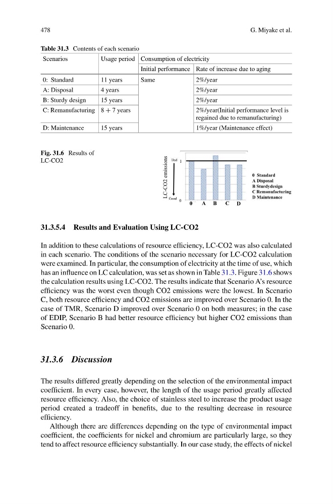
In addition to these calculations of resource efficiency, LC-CO2 was also calculated
in each scenario. The conditions of the scenario necessary for LC-CO2 calculation
were examined. In particular, the consumption of electricity at the time of use, which
has an influence on LC calculation, was set as shown in Table 31.3. Figure 31.6 shows
the calculation results using LC-CO2. The results indicate that Scenario A’s resource
efficiency was the worst even though CO2 emissions were the lowest. In Scenario
C, both resource efficiency and CO2 emissions are improved over Scenario 0. In the
case of TMR, Scenario D improved over Scenario 0 on both measures; in the case
of EDIP, Scenario B had better resource efficiency but higher CO2 emissions than
Scenario 0.
31.3.6 Discussion
The results differed greatly depending on the selection of the environmental impact
coefficient. In every case, however, the length of the usage period greatly affected
resource efficiency. Also, the choice of stainless steel to increase the product usage
period created a tradeoff in benefits, due to the resulting decrease in resource
efficiency.
Although there are differences depending on the type of environmental impact
coefficient, the coefficients for nickel and chromium are particularly large, so they
tend to affect resource efficiency substantially. In our case study, the effects of nickel
G. Miyake et al.
Table 31.3 Contents of each scenario
Scenarios
Usage period Consumption of electricity
Initial performance Rate of increase due to aging
0: Standard
11 years
Same
2%/year
A: Disposal
4 years
2%/year
B: Sturdy design
15 years
2%/year
C: Remanufacturing 8 + 7 years
2%/year(Initial performance level is
regained due to remanufacturing)
D: Maintenance
15 years
1%/year (Maintenance effect)
Fig. 31.6 Results of
LC-CO2
0.0
0.2
0.4
0.6
0.8
1.0
1.2
0ABCD
LC-CO2 emissions
1
0
A B
C D
0
Good
Bad
A Disposal
B Sturdydesign
C Remanufacturing
D Maintenance
0 Standard
31.3.5.4 Results and Evaluation Using LC-CO2
In addition to these calculations of resource efficiency, LC-CO2 was also calculated
in each scenario. The conditions of the scenario necessary for LC-CO2 calculation
were examined. In particular, the consumption of electricity at the time of use, which
has an influence on LC calculation, was set as shown in Table 31.3. Figure 31.6 shows
the calculation results using LC-CO2. The results indicate that Scenario A’s resource
efficiency was the worst even though CO2 emissions were the lowest. In Scenario
C, both resource efficiency and CO2 emissions are improved over Scenario 0. In the
case of TMR, Scenario D improved over Scenario 0 on both measures; in the case
of EDIP, Scenario B had better resource efficiency but higher CO2 emissions than
Scenario 0.
31.3.6 Discussion
The results differed greatly depending on the selection of the environmental impact
coefficient. In every case, however, the length of the usage period greatly affected
resource efficiency. Also, the choice of stainless steel to increase the product usage
period created a tradeoff in benefits, due to the resulting decrease in resource
efficiency.
Although there are differences depending on the type of environmental impact
coefficient, the coefficients for nickel and chromium are particularly large, so they
tend to affect resource efficiency substantially. In our case study, the effects of nickel