

6.7 Movement of Efimov States in 20 C Causing Resonance …
99
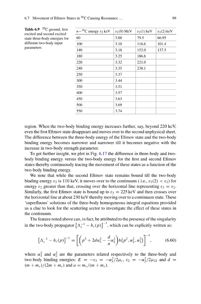
Table 6.9 20 C ground, first
excited and second excited
state three-body energies for
different two-body input
parameters
n− 18 C energy ε 2 keV ε 3 (0) MeV ε 3 (1) keV ε 3 (2) keV
60
3.00
79.5
66.95
100
3.10
116.6
101.4
140
3.18
152.0
137.5
180
3.25
186.6
220
3.32
221.0
240
3.35
238.1
250
3.37
300
3.44
350
3.51
400
3.57
450
3.63
500
3.69
550
3.74
region. When the two-body binding energy increases further, say, beyond 220 keV,
even the first Efimov state disappears and moves over to the second unphysical sheet.
The difference between the three-body energy of the Efimov state and the two-body
binding energy becomes narrower and narrower till it becomes negative with the
increase in two-body strength parameter.
To get further insight, we plot in Fig. 6.17 the difference in three-body and twobody binding energy versus the two-body energy for the first and second Efimov
states thereby continuously tracing the movement of these states as a function of the
two-body binding energy.
We note that while the second Efimov state remains bound till the two-body
binding energy ε 2 is 110 keV, it moves over to the continuum ( i.e., ε 3 (2) < ε 2 ) for
energy ε 2 greater than that, crossing over the horizontal line representing ε 3 = ε 2 .
Similarly, the first Efimov state is bound up to ε 3 = 225 keV and then crosses over
the horizontal line at about 230 keV thereby moving over to a continuum state. These
‘superfluous’ solutions of the three-body homogeneous integral equations provided
us a clue to look for the scattering sector to investigate the effect of these states in
the continuum.
The feature noted above can, in fact, be attributed to the presence of the singularity
in the two-body propagator
−1
c − h c ( p)
−1 , which can be explicitly written as:
−1
c − h c ( p)
−1 =
p
2
+ 2dα
2
3 −
d
a
α
2
2
h
p
2
, α
2
2 , α
2
3
−1
,
(6.60)
where α
2
3 and α
2
2 are the parameters related respectively to the three-body and
two-body binding energies: E = −ε 3 = −α
2
3 /2μ r , ε 2 = −α
2
2 /2μ 23 and d =
(m + m c )/(2m + m c ) and a = m c /(m + m c ).
99
Table 6.9 20 C ground, first
excited and second excited
state three-body energies for
different two-body input
parameters
n− 18 C energy ε 2 keV ε 3 (0) MeV ε 3 (1) keV ε 3 (2) keV
60
3.00
79.5
66.95
100
3.10
116.6
101.4
140
3.18
152.0
137.5
180
3.25
186.6
220
3.32
221.0
240
3.35
238.1
250
3.37
300
3.44
350
3.51
400
3.57
450
3.63
500
3.69
550
3.74
region. When the two-body binding energy increases further, say, beyond 220 keV,
even the first Efimov state disappears and moves over to the second unphysical sheet.
The difference between the three-body energy of the Efimov state and the two-body
binding energy becomes narrower and narrower till it becomes negative with the
increase in two-body strength parameter.
To get further insight, we plot in Fig. 6.17 the difference in three-body and twobody binding energy versus the two-body energy for the first and second Efimov
states thereby continuously tracing the movement of these states as a function of the
two-body binding energy.
We note that while the second Efimov state remains bound till the two-body
binding energy ε 2 is 110 keV, it moves over to the continuum ( i.e., ε 3 (2) < ε 2 ) for
energy ε 2 greater than that, crossing over the horizontal line representing ε 3 = ε 2 .
Similarly, the first Efimov state is bound up to ε 3 = 225 keV and then crosses over
the horizontal line at about 230 keV thereby moving over to a continuum state. These
‘superfluous’ solutions of the three-body homogeneous integral equations provided
us a clue to look for the scattering sector to investigate the effect of these states in
the continuum.
The feature noted above can, in fact, be attributed to the presence of the singularity
in the two-body propagator
−1
c − h c ( p)
−1 , which can be explicitly written as:
−1
c − h c ( p)
−1 =
p
2
+ 2dα
2
3 −
d
a
α
2
2
h
p
2
, α
2
2 , α
2
3
−1
,
(6.60)
where α
2
3 and α
2
2 are the parameters related respectively to the three-body and
two-body binding energies: E = −ε 3 = −α
2
3 /2μ r , ε 2 = −α
2
2 /2μ 23 and d =
(m + m c )/(2m + m c ) and a = m c /(m + m c ).