

92
6 Three-Body Approach to Structural Properties …
where μ n = π
2
λ n /β
3
1 and μ c = π
2
λ c /
2aβ
3
1
are now dimensionless strength
parameters. We also reduce the two coupled integral equations into one equation for
χ( p) by substituting Eq. (4.27) into (4.26) and using the definitions (6.51) for φ( p)
and χ( p) given above. Thus,
λ i χ( p) =
d q K 3 (
p,
q; ε)τ c (q)χ ( q)
+ 2
¨
d qd q
K 2 (
p,
q; ε)τ n (q)K 1
q,
q
; ε
τ c
q
χ
q
(6.54)
where the kernels K 1 , K 2 and K 3 are the same as given in Eq. (4.28) except that the
variables p, q, etc., are now dimensionless quantities:
p/β 1 → p and q/β 1 → q, and − m E/β
2
1 ≡ ε 3 , β r = β/β 1 .
(6.55)
The integral Eq. (6.54) is the eigenvalue equation in λ i . After having performed
the angular integration over the vectors − → q and − → q
and having symmetrized the
final kernel, we compute the integral equation as an eigenvalue equation in λ i .In
fact, by feeding the parameters of binary systems, i.e., for n–n and n–c potentials
in the right-hand side of Eq. (6.54), we seek the solution of the above equation for
the three-body binding energy parameter ε 3 when the eigenvalue λ i approaches 1,
accurate to at least four decimal places. Here, it may be pointed out that the factors
τ n and τ c defined through Eqs. (6.52) and (6.53) are quite sensitive particularly when
the scattering lengths of the binary sub-systems get infinitely large values. In fact,
these factors blow up as the variable p → 0 and the three-body energy parameter ε 3
approaches extremely small values. This necessitates, from the computational point
of view, a rather large size of the three-body matrix with double precision so as to
minimize the possible truncation errors.
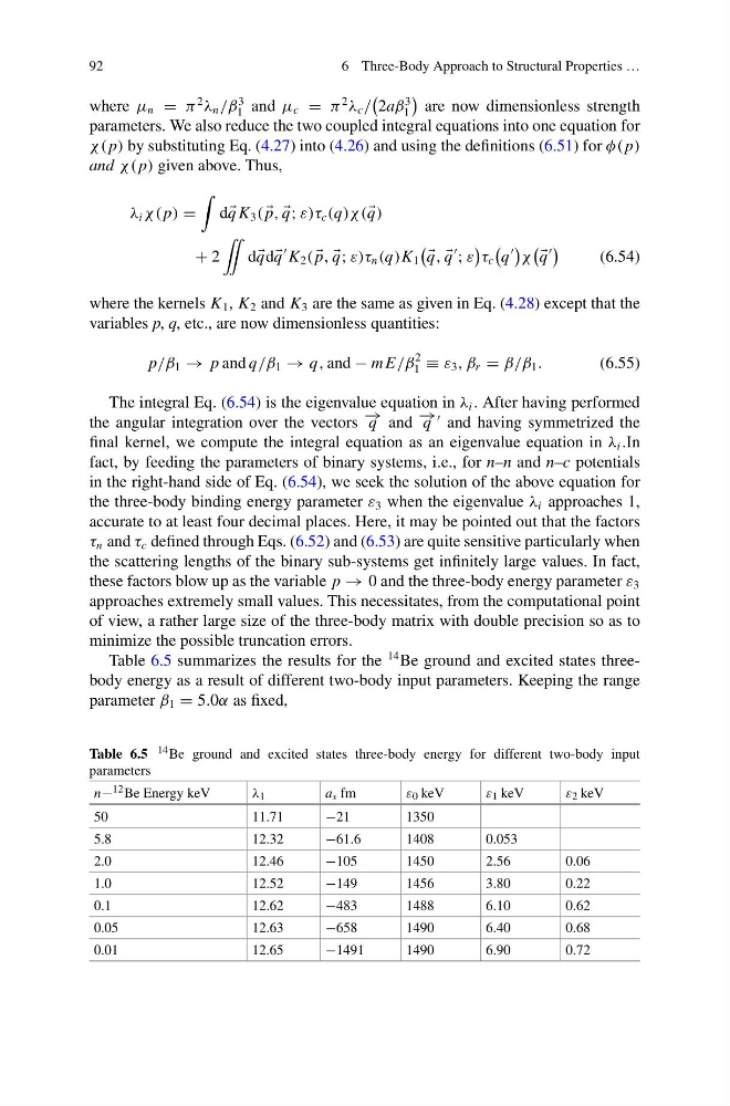
Table 6.5 summarizes the results for the
14 Be ground and excited states threebody energy as a result of different two-body input parameters. Keeping the range
parameter β 1 = 5.0α as fixed,
Table 6.5 14 Be ground and excited states three-body energy for different two-body input
parameters
n− 12 Be Energy keV
λ 1
a s fm
ε 0 keV
ε 1 keV
ε 2 keV
50
11.71
−21
1350
5.8
12.32
−61.6
1408
0.053
2.0
12.46
−105
1450
2.56
0.06
1.0
12.52
−149
1456
3.80
0.22
0.1
12.62
−483
1488
6.10
0.62
0.05
12.63
−658
1490
6.40
0.68
0.01
12.65
−1491
1490
6.90
0.72
6 Three-Body Approach to Structural Properties …
where μ n = π
2
λ n /β
3
1 and μ c = π
2
λ c /
2aβ
3
1
are now dimensionless strength
parameters. We also reduce the two coupled integral equations into one equation for
χ( p) by substituting Eq. (4.27) into (4.26) and using the definitions (6.51) for φ( p)
and χ( p) given above. Thus,
λ i χ( p) =
d q K 3 (
p,
q; ε)τ c (q)χ ( q)
+ 2
¨
d qd q
K 2 (
p,
q; ε)τ n (q)K 1
q,
q
; ε
τ c
q
χ
q
(6.54)
where the kernels K 1 , K 2 and K 3 are the same as given in Eq. (4.28) except that the
variables p, q, etc., are now dimensionless quantities:
p/β 1 → p and q/β 1 → q, and − m E/β
2
1 ≡ ε 3 , β r = β/β 1 .
(6.55)
The integral Eq. (6.54) is the eigenvalue equation in λ i . After having performed
the angular integration over the vectors − → q and − → q
and having symmetrized the
final kernel, we compute the integral equation as an eigenvalue equation in λ i .In
fact, by feeding the parameters of binary systems, i.e., for n–n and n–c potentials
in the right-hand side of Eq. (6.54), we seek the solution of the above equation for
the three-body binding energy parameter ε 3 when the eigenvalue λ i approaches 1,
accurate to at least four decimal places. Here, it may be pointed out that the factors
τ n and τ c defined through Eqs. (6.52) and (6.53) are quite sensitive particularly when
the scattering lengths of the binary sub-systems get infinitely large values. In fact,
these factors blow up as the variable p → 0 and the three-body energy parameter ε 3
approaches extremely small values. This necessitates, from the computational point
of view, a rather large size of the three-body matrix with double precision so as to
minimize the possible truncation errors.
Table 6.5 summarizes the results for the
14 Be ground and excited states threebody energy as a result of different two-body input parameters. Keeping the range
parameter β 1 = 5.0α as fixed,
Table 6.5 14 Be ground and excited states three-body energy for different two-body input
parameters
n− 12 Be Energy keV
λ 1
a s fm
ε 0 keV
ε 1 keV
ε 2 keV
50
11.71
−21
1350
5.8
12.32
−61.6
1408
0.053
2.0
12.46
−105
1450
2.56
0.06
1.0
12.52
−149
1456
3.80
0.22
0.1
12.62
−483
1488
6.10
0.62
0.05
12.63
−658
1490
6.40
0.68
0.01
12.65
−1491
1490
6.90
0.72