

B ¼ F 2 À 5F 4 C ¼ 35F 4
Still for the V(III) ion
E
3 P À
3 F
ð
Þ¼15F 2 À 75F 4 ¼ 13;000 cm
À1
E
1 D À
3 F
ð
Þ¼5F 2 þ 45F 4 ¼ 10;600 cm
À1
one obtains F 2 ¼ 1310 cm
À1 and F 4 ¼ 90 cm
À1 .
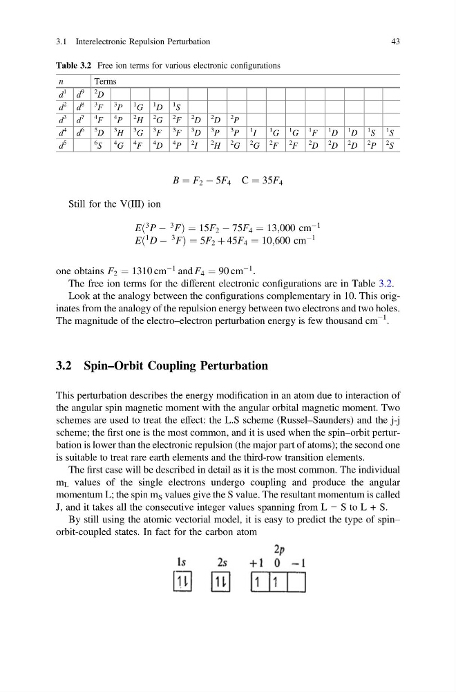
The free ion terms for the different electronic configurations are in Table 3.2.
Look at the analogy between the configurations complementary in 10. This originates from the analogy of the repulsion energy between two electrons and two holes.
The magnitude of the electro–electron perturbation energy is few thousand cm
−1 .
3.2 Spin–Orbit Coupling Perturbation
This perturbation describes the energy modification in an atom due to interaction of
the angular spin magnetic moment with the angular orbital magnetic moment. Two
schemes are used to treat the effect: the L.S scheme (Russel–Saunders) and the j-j
scheme; the first one is the most common, and it is used when the spin–orbit perturbation is lower than the electronic repulsion (the major part of atoms); the second one
is suitable to treat rare earth elements and the third-row transition elements.
The first case will be described in detail as it is the most common. The individual
m L values of the single electrons undergo coupling and produce the angular
momentum L; the spin m S values give the S value. The resultant momentum is called
J, and it takes all the consecutive integer values spanning from L − S to L + S.
By still using the atomic vectorial model, it is easy to predict the type of spin–
orbit-coupled states. In fact for the carbon atom
Table 3.2 Free ion terms for various electronic configurations
n
Terms
d
1
d
9
2
D
d
2
d
8
3
F
3
P
1
G
1
D
1
S
d
3
d
7
4
F
4
P
2
H
2
G
2
F
2
D
2
D
2
P
d
4
d
6
5
D
3
H
3
G
3
F
3
F
3
D
3
P
3
P
1
I
1
G
1
G
1
F
1
D
1
D
1
S
1
S
d
5
6
S
4
G
4
F
4
D
4
P
2
I
2
H
2
G
2
G
2
F
2
F
2
D
2
D
2
D
2
P
2
S
3.1 Interelectronic Repulsion Perturbation
43
Still for the V(III) ion
E
3 P À
3 F
ð
Þ¼15F 2 À 75F 4 ¼ 13;000 cm
À1
E
1 D À
3 F
ð
Þ¼5F 2 þ 45F 4 ¼ 10;600 cm
À1
one obtains F 2 ¼ 1310 cm
À1 and F 4 ¼ 90 cm
À1 .
The free ion terms for the different electronic configurations are in Table 3.2.
Look at the analogy between the configurations complementary in 10. This originates from the analogy of the repulsion energy between two electrons and two holes.
The magnitude of the electro–electron perturbation energy is few thousand cm
−1 .
3.2 Spin–Orbit Coupling Perturbation
This perturbation describes the energy modification in an atom due to interaction of
the angular spin magnetic moment with the angular orbital magnetic moment. Two
schemes are used to treat the effect: the L.S scheme (Russel–Saunders) and the j-j
scheme; the first one is the most common, and it is used when the spin–orbit perturbation is lower than the electronic repulsion (the major part of atoms); the second one
is suitable to treat rare earth elements and the third-row transition elements.
The first case will be described in detail as it is the most common. The individual
m L values of the single electrons undergo coupling and produce the angular
momentum L; the spin m S values give the S value. The resultant momentum is called
J, and it takes all the consecutive integer values spanning from L − S to L + S.
By still using the atomic vectorial model, it is easy to predict the type of spin–
orbit-coupled states. In fact for the carbon atom
Table 3.2 Free ion terms for various electronic configurations
n
Terms
d
1
d
9
2
D
d
2
d
8
3
F
3
P
1
G
1
D
1
S
d
3
d
7
4
F
4
P
2
H
2
G
2
F
2
D
2
D
2
P
d
4
d
6
5
D
3
H
3
G
3
F
3
F
3
D
3
P
3
P
1
I
1
G
1
G
1
F
1
D
1
D
1
S
1
S
d
5
6
S
4
G
4
F
4
D
4
P
2
I
2
H
2
G
2
G
2
F
2
F
2
D
2
D
2
D
2
P
2
S
3.1 Interelectronic Repulsion Perturbation
43