

where H 11 ¼ W
0
1 H
j jW
0
1
H 22 ¼ W
0
2 H
j jW
0
2
has H 11 and H 22 as solutions, when H 21 = H 12 ,
E 1 ¼ H ¼ W
0
1 H
0
þ H
0
W
0
1
¼ W
0
1 H
0
W
0
1
þ W
0
1 H
0
j jW
0
1
¼ E
0
1 þ W
0
1 H
0
j jW
0
1
E 2 ¼ H 22 ¼ E
0
2 þ W
0
2 H
0
j jW
0
2
In a similar way as in the case of LCAO method, it is still a great difficulty to
exactly calculate the H ij integrals. We will evaluate them by a semiempirical
method, using the experimental parameters taken from the spectroscopic
measurements.
The perturbation method can be positively applied when the perturbation energy
is well lower than the energies of the unperturbed system, and it never suitably
describes the covalent bond.
Based on this assumption, in the following, we will describe the perturbations
that modellize the atomic electronic structure.
3.1 Interelectronic Repulsion Perturbation
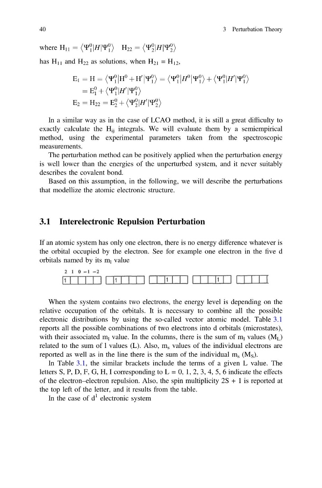
If an atomic system has only one electron, there is no energy difference whatever is
the orbital occupied by the electron. See for example one electron in the five d
orbitals named by its m l value
When the system contains two electrons, the energy level is depending on the
relative occupation of the orbitals. It is necessary to combine all the possible
electronic distributions by using the so-called vector atomic model. Table 3.1
reports all the possible combinations of two electrons into d orbitals (microstates),
with their associated m l value. In the columns, there is the sum of m l values (M L )
related to the sum of l values (L). Also, m s values of the individual electrons are
reported as well as in the line there is the sum of the individual m s (M S ).
In Table 3.1, the similar brackets include the terms of a given L value. The
letters S, P, D, F, G, H, I corresponding to L = 0, 1, 2, 3, 4, 5, 6 indicate the effects
of the electron–electron repulsion. Also, the spin multiplicity 2S + 1 is reported at
the top left of the letter, and it results from the table.
In the case of d
1 electronic system
40
3 Perturbation Theory
0
1 H
j jW
0
1
H 22 ¼ W
0
2 H
j jW
0
2
has H 11 and H 22 as solutions, when H 21 = H 12 ,
E 1 ¼ H ¼ W
0
1 H
0
þ H
0
W
0
1
¼ W
0
1 H
0
W
0
1
þ W
0
1 H
0
j jW
0
1
¼ E
0
1 þ W
0
1 H
0
j jW
0
1
E 2 ¼ H 22 ¼ E
0
2 þ W
0
2 H
0
j jW
0
2
In a similar way as in the case of LCAO method, it is still a great difficulty to
exactly calculate the H ij integrals. We will evaluate them by a semiempirical
method, using the experimental parameters taken from the spectroscopic
measurements.
The perturbation method can be positively applied when the perturbation energy
is well lower than the energies of the unperturbed system, and it never suitably
describes the covalent bond.
Based on this assumption, in the following, we will describe the perturbations
that modellize the atomic electronic structure.
3.1 Interelectronic Repulsion Perturbation
If an atomic system has only one electron, there is no energy difference whatever is
the orbital occupied by the electron. See for example one electron in the five d
orbitals named by its m l value
When the system contains two electrons, the energy level is depending on the
relative occupation of the orbitals. It is necessary to combine all the possible
electronic distributions by using the so-called vector atomic model. Table 3.1
reports all the possible combinations of two electrons into d orbitals (microstates),
with their associated m l value. In the columns, there is the sum of m l values (M L )
related to the sum of l values (L). Also, m s values of the individual electrons are
reported as well as in the line there is the sum of the individual m s (M S ).
In Table 3.1, the similar brackets include the terms of a given L value. The
letters S, P, D, F, G, H, I corresponding to L = 0, 1, 2, 3, 4, 5, 6 indicate the effects
of the electron–electron repulsion. Also, the spin multiplicity 2S + 1 is reported at
the top left of the letter, and it results from the table.
In the case of d
1 electronic system
40
3 Perturbation Theory