

E1C03 09/14/2010
15:24:52 Page 82
and subject to a general input signal, represented by the forcing function, F(t):
a n
d
n
y
dt n þ a nÀ1
d
nÀ1
y
dt nÀ1 þ Á Á Á þ a 1
dy
dt
þ a 0 y ¼ F t
ð Þ
ð3:1Þ
where
F t
ð Þ ¼ b m
d
m
x
dt m þ b mÀ1
d
mÀ1
x
dt mÀ1 þ Á Á Á þ b 1
dx
dt
þ b 0 x m n
The coefficients a 0 , a 1 , a 2 , . . . , a n and b 0 , b 1 , . . . , b m represent physical system parameters whose
properties and values depend on the measurement system itself. Real measurement systems can be
modeled this way by considering their governing system equations. These equations are generated
by application of pertinent fundamental physical laws of nature to the measurement system. Our
discussion is limited to measurement system concepts, but a general treatment of systems can be
found in text books dedicated to that topic (1–3).
Example 3.1
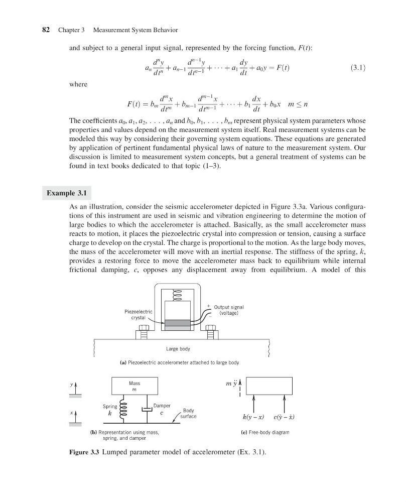
As an illustration, consider the seismic accelerometer depicted in Figure 3.3a. Various configurations of this instrument are used in seismic and vibration engineering to determine the motion of
large bodies to which the accelerometer is attached. Basically, as the small accelerometer mass
reacts to motion, it places the piezoelectric crystal into compression or tension, causing a surface
charge to develop on the crystal. The charge is proportional to the motion. As the large body moves,
the mass of the accelerometer will move with an inertial response. The stiffness of the spring, k,
provides a restoring force to move the accelerometer mass back to equilibrium while internal
frictional damping, c, opposes any displacement away from equilibrium. A model of this
(a) Piezoelectric accelerometer attached to large body
(b) Representation using mass,
spring, and damper
(c) Free-body diagram
c(y – x)
k(y – x)
Mass
m
Spring
k
Damper
c
Body
surface
y
x
Piezoelectric
crystal
Output signal
(voltage)
Large body
+
–
m y
.
.
..
Figure 3.3 Lumped parameter model of accelerometer (Ex. 3.1).
82 Chapter 3 Measurement System Behavior
15:24:52 Page 82
and subject to a general input signal, represented by the forcing function, F(t):
a n
d
n
y
dt n þ a nÀ1
d
nÀ1
y
dt nÀ1 þ Á Á Á þ a 1
dy
dt
þ a 0 y ¼ F t
ð Þ
ð3:1Þ
where
F t
ð Þ ¼ b m
d
m
x
dt m þ b mÀ1
d
mÀ1
x
dt mÀ1 þ Á Á Á þ b 1
dx
dt
þ b 0 x m n
The coefficients a 0 , a 1 , a 2 , . . . , a n and b 0 , b 1 , . . . , b m represent physical system parameters whose
properties and values depend on the measurement system itself. Real measurement systems can be
modeled this way by considering their governing system equations. These equations are generated
by application of pertinent fundamental physical laws of nature to the measurement system. Our
discussion is limited to measurement system concepts, but a general treatment of systems can be
found in text books dedicated to that topic (1–3).
Example 3.1
As an illustration, consider the seismic accelerometer depicted in Figure 3.3a. Various configurations of this instrument are used in seismic and vibration engineering to determine the motion of
large bodies to which the accelerometer is attached. Basically, as the small accelerometer mass
reacts to motion, it places the piezoelectric crystal into compression or tension, causing a surface
charge to develop on the crystal. The charge is proportional to the motion. As the large body moves,
the mass of the accelerometer will move with an inertial response. The stiffness of the spring, k,
provides a restoring force to move the accelerometer mass back to equilibrium while internal
frictional damping, c, opposes any displacement away from equilibrium. A model of this
(a) Piezoelectric accelerometer attached to large body
(b) Representation using mass,
spring, and damper
(c) Free-body diagram
c(y – x)
k(y – x)
Mass
m
Spring
k
Damper
c
Body
surface
y
x
Piezoelectric
crystal
Output signal
(voltage)
Large body
+
–
m y
.
.
..
Figure 3.3 Lumped parameter model of accelerometer (Ex. 3.1).
82 Chapter 3 Measurement System Behavior