

E1C02 09/14/2010
13:35:19 Page 67
FIND {y(rdt)}
SOLUTION Measuring y(t) every 0.125 s over 1 s produces the discrete data set {y(rdt)} given
in Table 2.2. Note that the measurement produces four complete periods of the signal and that the
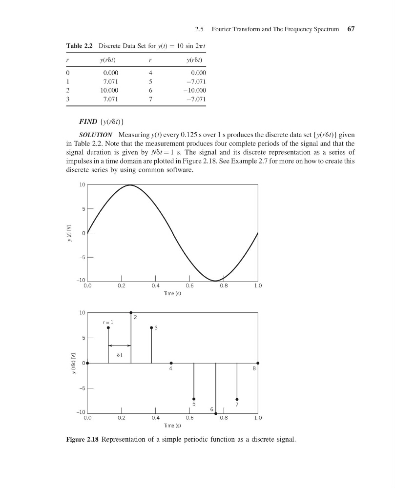
signal duration is given by Ndt ¼ 1 s. The signal and its discrete representation as a series of
impulses in a time domain are plotted in Figure 2.18. See Example 2.7 for more on how to create this
discrete series by using common software.
Table 2.2 Discrete Data Set for y(t) ¼ 10 sin 2pt
r
y (rdt)
r
y (rdt)
0
0.000
4
0.000
1
7.071
5
À7.071
2
10.000
6
À10.000
3
7.071
7
À7.071
10
5
0
–5
–10
0.2
2
3
8
4
5
6
7
1.0
0.8
0.6
0.4
0.0
–10
–5
0
5
10
Time (s)
r = 1
y (rδt) [V]
y (t) [V]
0.2
1.0
0.8
0.6
0.4
0.0
Time (s)
δ t
Figure 2.18 Representation of a simple periodic function as a discrete signal.
2.5 Fourier Transform and The Frequency Spectrum 67
13:35:19 Page 67
FIND {y(rdt)}
SOLUTION Measuring y(t) every 0.125 s over 1 s produces the discrete data set {y(rdt)} given
in Table 2.2. Note that the measurement produces four complete periods of the signal and that the
signal duration is given by Ndt ¼ 1 s. The signal and its discrete representation as a series of
impulses in a time domain are plotted in Figure 2.18. See Example 2.7 for more on how to create this
discrete series by using common software.
Table 2.2 Discrete Data Set for y(t) ¼ 10 sin 2pt
r
y (rdt)
r
y (rdt)
0
0.000
4
0.000
1
7.071
5
À7.071
2
10.000
6
À10.000
3
7.071
7
À7.071
10
5
0
–5
–10
0.2
2
3
8
4
5
6
7
1.0
0.8
0.6
0.4
0.0
–10
–5
0
5
10
Time (s)
r = 1
y (rδt) [V]
y (t) [V]
0.2
1.0
0.8
0.6
0.4
0.0
Time (s)
δ t
Figure 2.18 Representation of a simple periodic function as a discrete signal.
2.5 Fourier Transform and The Frequency Spectrum 67