

E1C02 09/14/2010
13:35:19 Page 65
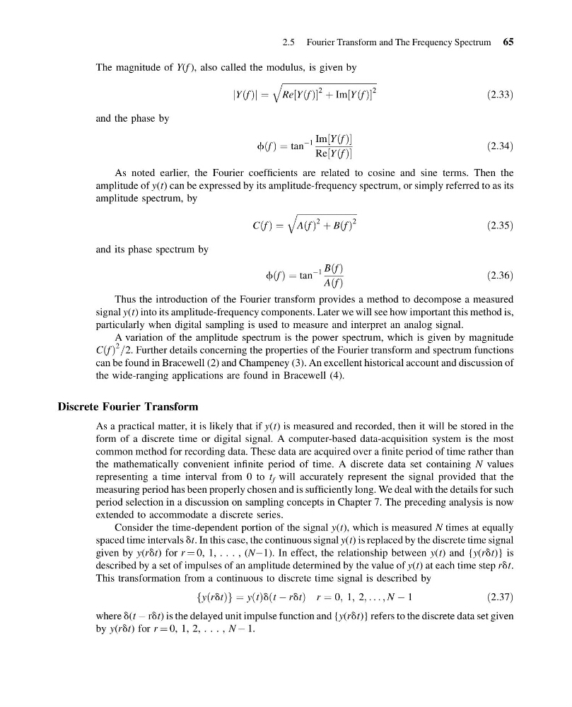
The magnitude of Y(f ), also called the modulus, is given by
jY f
ð Þj ¼
ffiffiffiffiffiffiffiffiffiffiffiffiffiffiffiffiffiffiffiffiffiffiffiffiffiffiffiffiffiffiffiffiffiffiffiffiffiffiffiffiffiffiffi
Re Y f
ð Þ
½
2 þ Im Y f
ð Þ
½
2
q
ð2:33Þ
and the phase by
f f
ð Þ ¼ tan
À1 Im Y f
ð Þ
½
Re Y f
ð Þ
½
ð2:34Þ
As noted earlier, the Fourier coefficients are related to cosine and sine terms. Then the
amplitude of y(t) can be expressed by its amplitude-frequency spectrum, or simply referred to as its
amplitude spectrum, by
C f
ð Þ ¼
ffiffiffiffiffiffiffiffiffiffiffiffiffiffiffiffiffiffiffiffiffiffiffiffiffiffiffi ffi
A f
ð Þ
2 þ B f
ð Þ
2
q
ð2:35Þ
and its phase spectrum by
f f
ð Þ ¼ tan
À1 B f
ð Þ
A f
ð Þ
ð2:36Þ
Thus the introduction of the Fourier transform provides a method to decompose a measured
signal y(t) into its amplitude-frequency components. Later we will see how important this method is,
particularly when digital sampling is used to measure and interpret an analog signal.
A variation of the amplitude spectrum is the power spectrum, which is given by magnitude
C f
ð Þ
2 =2. Further details concerning the properties of the Fourier transform and spectrum functions
can be found in Bracewell (2) and Champeney (3). An excellent historical account and discussion of
the wide-ranging applications are found in Bracewell (4).
Discrete Fourier Transform
As a practical matter, it is likely that if y(t) is measured and recorded, then it will be stored in the
form of a discrete time or digital signal. A computer-based data-acquisition system is the most
common method for recording data. These data are acquired over a finite period of time rather than
the mathematically convenient infinite period of time. A discrete data set containing N values
representing a time interval from 0 to t f will accurately represent the signal provided that the
measuring period has been properly chosen and is sufficiently long. We deal with the details for such
period selection in a discussion on sampling concepts in Chapter 7. The preceding analysis is now
extended to accommodate a discrete series.
Consider the time-dependent portion of the signal y(t), which is measured N times at equally
spaced time intervals dt. In this case, the continuous signal y(t) is replaced by the discrete time signal
given by y(rdt) for r ¼ 0, 1, . . . , (NÀ1). In effect, the relationship between y(t) and {y(rdt)} is
described by a set of impulses of an amplitude determined by the value of y(t) at each time step rdt.
This transformation from a continuous to discrete time signal is described by
y rdt
ð Þ
f
g¼ y t
ð Þd t À rdt
ð
Þ r ¼ 0; 1; 2; . . . ; N À 1
ð2:37Þ
where d(t À rdt) is the delayed unit impulse function and {y(rdt)} refers to the discrete data set given
by y(rdt) for r ¼ 0, 1, 2, . . . , N À 1.
2.5 Fourier Transform and The Frequency Spectrum 65
13:35:19 Page 65
The magnitude of Y(f ), also called the modulus, is given by
jY f
ð Þj ¼
ffiffiffiffiffiffiffiffiffiffiffiffiffiffiffiffiffiffiffiffiffiffiffiffiffiffiffiffiffiffiffiffiffiffiffiffiffiffiffiffiffiffiffi
Re Y f
ð Þ
½
2 þ Im Y f
ð Þ
½
2
q
ð2:33Þ
and the phase by
f f
ð Þ ¼ tan
À1 Im Y f
ð Þ
½
Re Y f
ð Þ
½
ð2:34Þ
As noted earlier, the Fourier coefficients are related to cosine and sine terms. Then the
amplitude of y(t) can be expressed by its amplitude-frequency spectrum, or simply referred to as its
amplitude spectrum, by
C f
ð Þ ¼
ffiffiffiffiffiffiffiffiffiffiffiffiffiffiffiffiffiffiffiffiffiffiffiffiffiffiffi ffi
A f
ð Þ
2 þ B f
ð Þ
2
q
ð2:35Þ
and its phase spectrum by
f f
ð Þ ¼ tan
À1 B f
ð Þ
A f
ð Þ
ð2:36Þ
Thus the introduction of the Fourier transform provides a method to decompose a measured
signal y(t) into its amplitude-frequency components. Later we will see how important this method is,
particularly when digital sampling is used to measure and interpret an analog signal.
A variation of the amplitude spectrum is the power spectrum, which is given by magnitude
C f
ð Þ
2 =2. Further details concerning the properties of the Fourier transform and spectrum functions
can be found in Bracewell (2) and Champeney (3). An excellent historical account and discussion of
the wide-ranging applications are found in Bracewell (4).
Discrete Fourier Transform
As a practical matter, it is likely that if y(t) is measured and recorded, then it will be stored in the
form of a discrete time or digital signal. A computer-based data-acquisition system is the most
common method for recording data. These data are acquired over a finite period of time rather than
the mathematically convenient infinite period of time. A discrete data set containing N values
representing a time interval from 0 to t f will accurately represent the signal provided that the
measuring period has been properly chosen and is sufficiently long. We deal with the details for such
period selection in a discussion on sampling concepts in Chapter 7. The preceding analysis is now
extended to accommodate a discrete series.
Consider the time-dependent portion of the signal y(t), which is measured N times at equally
spaced time intervals dt. In this case, the continuous signal y(t) is replaced by the discrete time signal
given by y(rdt) for r ¼ 0, 1, . . . , (NÀ1). In effect, the relationship between y(t) and {y(rdt)} is
described by a set of impulses of an amplitude determined by the value of y(t) at each time step rdt.
This transformation from a continuous to discrete time signal is described by
y rdt
ð Þ
f
g¼ y t
ð Þd t À rdt
ð
Þ r ¼ 0; 1; 2; . . . ; N À 1
ð2:37Þ
where d(t À rdt) is the delayed unit impulse function and {y(rdt)} refers to the discrete data set given
by y(rdt) for r ¼ 0, 1, 2, . . . , N À 1.
2.5 Fourier Transform and The Frequency Spectrum 65